Build an InSituData object from scratch#
from pathlib import Path
from insitupy import read_xenium
from datetime import datetime
from typing import Literal
import shutil
import pandas as pd
import numpy as np
import seaborn as sns
import matplotlib.pyplot as plt
import anndata as ad
import geopandas as gpd
import dask.array as da
from shapely.geometry import Polygon
from insitupy import InSituData
from insitupy._core.dataclasses import CellData, BoundariesData, ImageData, AnnotationsData, RegionsData
import cv2
import zarr
Let’s start by generating main modalities and adding them into InSituData#
Below you can find all functions used to generate the dummy code
# Function to generate a random H&E-like image
def generate_random_he_image(width, height):
    # Hematoxylin (blue-purple) and Eosin (pink) color ranges
    hematoxylin_color = np.array([102, 51, 153], dtype=np.uint8)  # Scaled to 0-255 range
    eosin_color = np.array([255, 204, 204], dtype=np.uint8)  # Scaled to 0-255 range
    # hematoxylin_color = np.array([0.4, 0.2, 0.6])
    # eosin_color = np.array([1.0, 0.8, 0.8])

    # random_image = np.random.rand(width, height, 3)
    random_image = np.random.randint(0, 256, (width, height, 3), dtype=np.uint8)
    he_image = random_image * hematoxylin_color // 255 + (255 - random_image) * eosin_color // 255
    # he_image = random_image * hematoxylin_color + (1 - random_image) * eosin_color

    return he_image

# Function to generate a random grayscale DAPI-like image
def generate_random_dapi_image(width, height):
    # DAPI (blue) color range in grayscale
    dapi_color = np.array([0.1, 0.1, 0.8])

    random_image = np.random.rand(width, height)
    dapi_image = random_image * dapi_color[2]  # Use the blue channel for grayscale

    return dapi_image

def generate_dummy_anndata(
    width,
    height,
    n_cells,
    num_genes = 400,
    pixel_size = 0.2125
    ):
    # In the next step we generate an `AnnData` object with respective spatial coordinates and a `Dask` Array with cellular boundaries for the respective cells.
    pixel_coordinates = np.random.rand(n_cells, 2) * [width, height]

    # Convert pixel coordinates to micrometers (1 pixel = 0.2125 micrometers)
    micrometer_coordinates = pixel_coordinates * pixel_size

    # Generate random gene expression counts matrix (n_cells x num_genes)
    gene_counts = np.random.poisson(lam=5, size=(n_cells, num_genes))

    # Create an AnnData object with gene expression counts and spatial coordinates
    adata = ad.AnnData(X=gene_counts)
    adata.obsm['spatial'] = micrometer_coordinates
    # Example observations (metadata)
    obs_data = {
        'cell_type': ['type1', 'type2'] * (n_cells // 2),  # Example cell types
        'batch': ['batch1'] * (n_cells // 2) + ['batch2'] * (n_cells // 2)  # Example batch information
    }

    # Add observations to the obs attribute
    adata.obs = adata.obs.assign(**obs_data)

    # add cell names
    adata.obs_names = [str(elem) for elem in range(1, n_cells+1)]
    return adata

def generate_cellular_boundaries_array(width, height, cell_positions, pixel_size, cell_size):
    # Create an empty mask
    mask = np.zeros((height, width), dtype=np.uint8)

    # Create random roundish shapes
    seg_mask_value = []
    for i, (x, y) in enumerate(cell_positions/pixel_size):
        num_points = np.random.randint(5, 15)  # Random number of points
        points = np.random.randint(-cell_size, cell_size, (num_points, 2)) + [x, y]
        hull = cv2.convexHull(points.astype(np.int32))
        value = i+1
        cv2.fillConvexPoly(mask, hull, value)
        seg_mask_value.append(value)

    # Convert the NumPy array to a Dask array with chunks
    dask_array = da.from_array(mask, chunks=(50, 50))

    return dask_array, seg_mask_value

# Function to generate random polygons
def generate_random_geometries(num_polygons, x_size, y_size, pixel_size, mode: Literal["region", "annotation"]):
    polygons = []
    attempts = 0
    max_attempts = num_polygons * 10  # Limit the number of attempts to avoid infinite loop

    while len(polygons) < num_polygons and attempts < max_attempts:
        # Generate random center point
        center_x = np.random.uniform(0, x_size*pixel_size)
        center_y = np.random.uniform(0, y_size*pixel_size)

        # Generate random size for the polygon
        size = np.random.uniform(10, 20)

        # Create a square polygon around the center point
        polygon = Polygon([
            (center_x - size, center_y - size),
            (center_x + size, center_y - size),
            (center_x + size, center_y + size),
            (center_x - size, center_y + size)
        ])

        # Check if the new polygon intersects with any existing polygons
        if not any(polygon.intersects(existing_polygon) for existing_polygon in polygons):
            polygons.append(polygon)

        attempts += 1

    if mode == "annotation":
        # Create GeoDataFrame with random polygons
        result_df = gpd.GeoDataFrame(geometry=polygons)
        result_df["id"] = result_df.index
        result_df["name"] = ['annotation1'] * (num_polygons // 2) + ['annotation2'] * (num_polygons - (num_polygons // 2))

    if mode == "region":
        # Create GeoDataFrame with random polygons
        result_df = gpd.GeoDataFrame(geometry=polygons)
        result_df["id"] = result_df.index
        result_df["name"] = result_df.index

    return result_df

# Function to generate a random H&E-like image with a scale of 0-255 and uint8
def generate_random_he_image(height, width):
    # Hematoxylin (blue-purple) and Eosin (pink) color ranges in 0-255 scale
    hematoxylin_color = np.array([102, 51, 153])
    eosin_color = np.array([255, 204, 204])

    random_image = np.random.rand(height, width, 3)
    he_image = random_image * hematoxylin_color + (1 - random_image) * eosin_color

    # Convert the image to uint8
    he_image_uint8 = he_image.astype(np.uint8)

    return he_image_uint8
def generate_random_grayscale_image(height, width):
    # Generate a random grayscale image
    random_image = np.random.rand(height, width) * 255

    # Convert the image to uint8
    grayscale_image_uint8 = random_image.astype(np.uint8)

    return grayscale_image_uint8
Now we use these functions to set up the dummy dataset step by step#
First we specify the parameters for the dummy dataset
# parameters
pixel_size = 0.2125
height_um = 100 # µm
width_um = 100 # µm
height = int(height_um / pixel_size) # pixel width
width = int(width_um / pixel_size) # pixel width
n_cells = 10
num_genes = 20
cell_size = 50
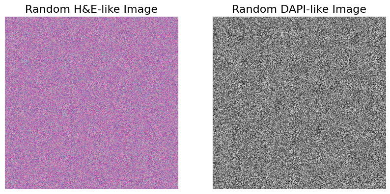
First, let’s generate an H&E-like random numpy image#
# Example usage
he_image = generate_random_he_image(height, width)
# Example usage
dapi_image = generate_random_grayscale_image(height, width)
# Display the generated images
plt.figure(figsize=(10, 5))

plt.subplot(1, 2, 1)
plt.imshow(he_image)
plt.title("Random H&E-like Image")
plt.axis('off')

plt.subplot(1, 2, 2)
plt.imshow(dapi_image, cmap='gray')
plt.title("Random DAPI-like Image")
plt.axis('off')

plt.show()
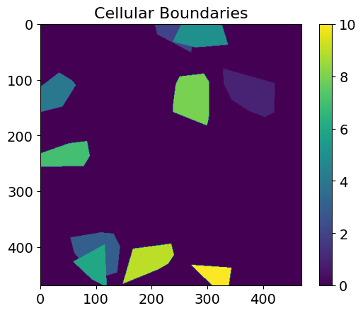
In the next step we generate an AnnData object with respective spatial coordinates and a Dask Array with cellular boundaries for the respective cells.#
The segmentation mask is a 2D array with 0 as background value and values ascending from 1 for each individual cell. The seg_mask_value variable is a list of these integer values and connects the names of the cells found in adata.obs_names with their corresponding value in the segmentation mask.
# generate random anndata
adata = generate_dummy_anndata(width=width, height=height, n_cells=n_cells, num_genes=num_genes, pixel_size=pixel_size)
# generate random boundaries mask
cellular_boundaries_array, seg_mask_value = generate_cellular_boundaries_array(
    width=width, height=height,
    cell_positions=adata.obsm["spatial"],
    pixel_size=pixel_size, cell_size=cell_size)
seg_mask_value
[1, 2, 3, 4, 5, 6, 7, 8, 9, 10]
# Plot the boundaries
plt.imshow(cellular_boundaries_array, cmap='viridis')
plt.title("Cellular Boundaries")
plt.colorbar()
plt.show()
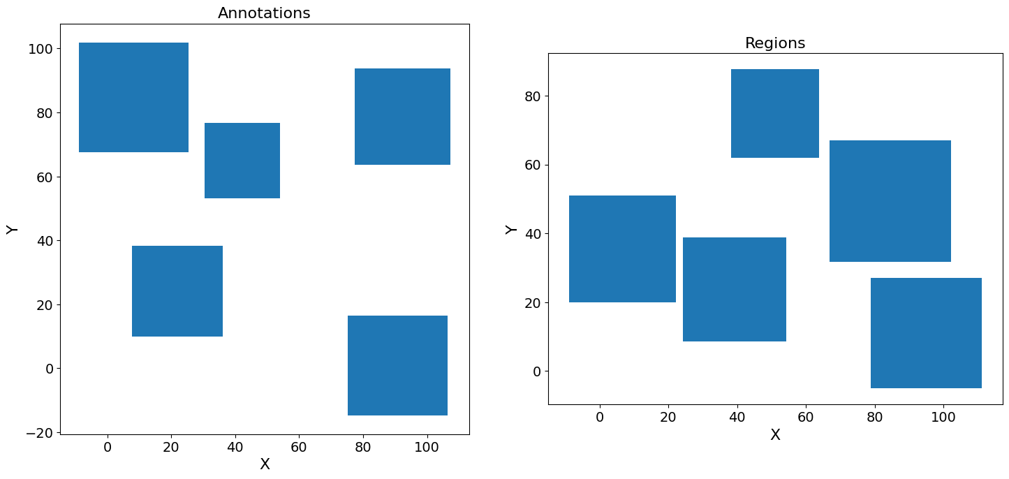
Let’s also generate example annotations and regions#
# generate random annotations and regions
gdf_annotations = generate_random_geometries(num_polygons=5, x_size=height, y_size=width, pixel_size=pixel_size, mode="annotation")
gdf_regions = generate_random_geometries(num_polygons=5, x_size=height, y_size=width, pixel_size=pixel_size, mode="region")
# Plot the annotations and regions
fig, axes = plt.subplots(nrows=1, ncols=2, figsize=(15, 7))

gdf_annotations.plot(ax=axes[0])
axes[0].set_title("Annotations")
axes[0].set_xlabel("X")
axes[0].set_ylabel("Y")

gdf_regions.plot(ax=axes[1])
axes[1].set_title("Regions")
axes[1].set_xlabel("X")
axes[1].set_ylabel("Y")

plt.tight_layout()
plt.show()
# Print the GeoDataFrame with random polygons
print(gdf_annotations.head())
print(gdf_regions.head())
                                            geometry  id         name
0  POLYGON ((75.246 -14.762, 106.494 -14.762, 106...   0  annotation1
1  POLYGON ((30.345 53.105, 54.057 53.105, 54.057...   1  annotation1
2  POLYGON ((77.415 63.742, 107.343 63.742, 107.3...   2  annotation2
3  POLYGON ((-8.899 67.629, 25.416 67.629, 25.416...   3  annotation2
4  POLYGON ((7.800 9.860, 36.175 9.860, 36.175 38...   4  annotation2
                                            geometry  id  name
0  POLYGON ((38.18516 61.96912, 63.87384 61.96912...   0     0
1  POLYGON ((78.84370 -5.10496, 111.06761 -5.1049...   1     1
2  POLYGON ((66.92718 31.70925, 102.12601 31.7092...   2     2
3  POLYGON ((24.17278 8.66402, 54.30960 8.66402, ...   3     3
4  POLYGON ((-8.91338 19.91125, 22.10692 19.91125...   4     4
Finally we create an InSituData object with all the modalities we have generated before#
xd = InSituData(
    path=Path("dummy_path"),
    metadata={
        "method": "Xenium"
              },
    slide_id="slide",
    sample_id="sample_1",
    from_insitudata=False
    )
xd
InSituData
Method:		Xenium
Slide ID:	slide
Sample ID:	sample_1
Path:		dummy_path
Metadata file:	None

No modalities loaded.
Then we add the data in the correct format. A CellData object consists of (i) the transcriptomic data as AnnData object and (ii) the cellular and/or nuclear boundaries as BoundariesData object.
# set up the boundaries data object
bd = BoundariesData(cell_names=adata.obs_names.astype(str), seg_mask_value=seg_mask_value)
bd.add_boundaries(data={"cellular": cellular_boundaries_array}, pixel_size=pixel_size)

# set up the object for the cellular data based on the anndata object and the boundaries object
cd = CellData(matrix=adata, boundaries=bd)
xd.cells = cd
Images are stored in an ImageData object:
# add an empty ImageData object and add the generated images
xd.images = ImageData()
xd.images.add_image(image=he_image, name="H&E", axes="xyc", pixel_size=pixel_size, ome_meta={'PhysicalSizeX': pixel_size})
xd.images.add_image(image=dapi_image, name="nuclei", axes="xyc", pixel_size=pixel_size, ome_meta={'PhysicalSizeX': pixel_size})
… and annotations and regions as AnnotationsData or RegionsData, respectively.
# add the annotations and regions data
xd.annotations = AnnotationsData()
xd.annotations.add_data(gdf_annotations, key="example_annotation", scale_factor=1)

xd.regions = RegionsData()
xd.regions.add_data(gdf_regions, key="example_regions", scale_factor=1)
xd
InSituData
Method:		Xenium
Slide ID:	slide
Sample ID:	sample_1
Path:		dummy_path
Metadata file:	None
    ➤ images
       H&E:	(470, 470, 3)
       nuclei:	(470, 470)
    ➤ cells
       matrix
           AnnData object with n_obs × n_vars = 10 × 20
           obs: 'cell_type', 'batch'
           obsm: 'spatial'
       boundaries
           BoundariesData object with 1 entry:
               cellular
    ➤ annotations
       example_annotation:	5 annotations, 2 classes ('annotation1','annotation2')
    ➤ regions
       example_regions:	5 regions, 5 classes ('0','1','2','3','4')
Save the data into an InSituPy project#
savepath = 'out/dummy_data'
xd.saveas(savepath, overwrite=True)
Saving data to out\dummy_data
Saved.
Reload data#
xd = InSituData.read(savepath)
xd.load_all()
Visualize the data using the napari-viewer#
xd.show()