Differential gene expression analysis for publication Figure 4#
Plan for publication#
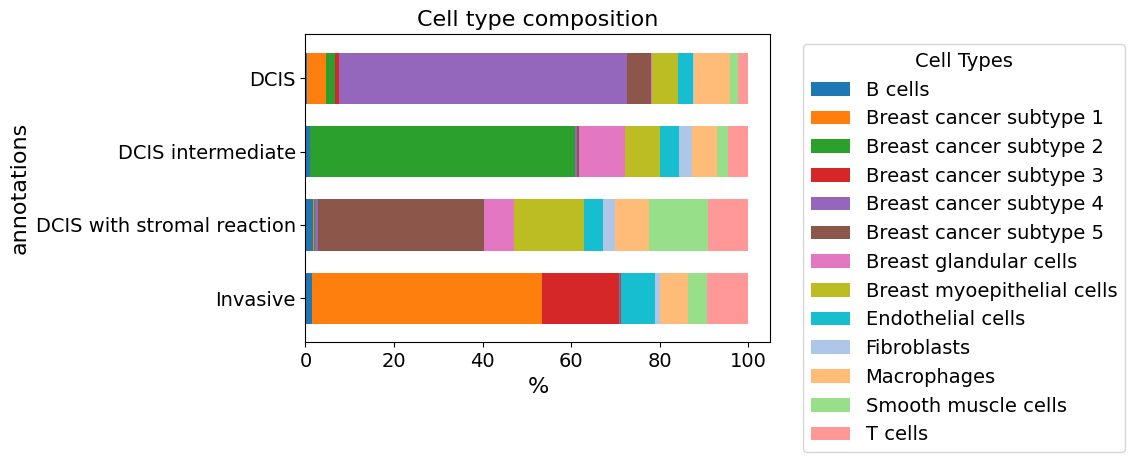
Use Katja’s descriptions/annotations to specify the identity of the 5 subtypes: plot the cell composition within each annotation (stroma enriched DCIS vs normal DCIS vs intermediate DCIS vs. invasive)
Differential gene expression analysis between DCIS and invasive (for this the comparison of two different cell types needs to be implemented)
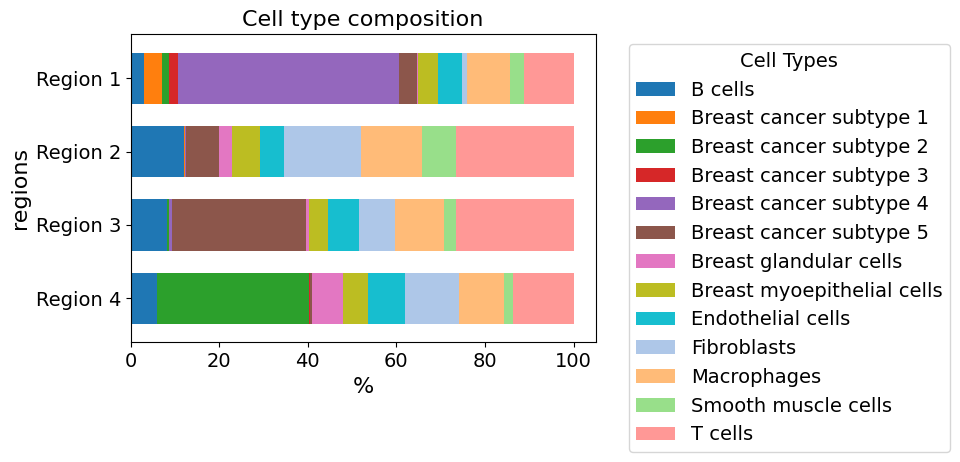
Analyze regions to show the stromal enrichment of Region 2, 3 and 4 compared to Region 1 which is non-stroma-enriched DCIS (which can be also seen in transcriptome)
from pathlib import Path
from insitupy import InSituData, CACHE
from insitupy.plotting import plot_cellular_composition
import warnings
warnings.simplefilter(action='ignore', category=FutureWarning)
Load Xenium data into InSituData object#
Now the Xenium data can be parsed by providing the data path to the InSituPy project folder.
insitupy_project = Path(CACHE / "out/demo_insitupy_project")
xd = InSituData.read(insitupy_project)
xd.load_all()
xd.import_annotations(
    files=r"C:\Users\ge37voy\Github\InSituPy\notebooks\demo_annotations\breast_cancer_annotations_publ.geojson",
    keys="Janesick",
    scale_factor=0.2125
)
xd.import_annotations(
    files=r"C:\Users\ge37voy\Github\InSituPy\notebooks\demo_annotations\breast_cancer_annotations_Katja.geojson",
    keys="Katja",
    scale_factor=0.2125
)
xd.import_regions(
    files=r"C:\Users\ge37voy\Github\InSituPy\notebooks\demo_annotations\breast_cancer_regions_Katja.geojson",
    keys="Katja",
    scale_factor=0.2125
)
xd
InSituData
Method:		Xenium
Slide ID:	0001879
Sample ID:	Replicate 1
Path:		C:\Users\ge37voy\.cache\InSituPy\out\demo_insitupy_project
Metadata file:	.ispy
    ➤ images
       nuclei:	(25778, 35416)
       CD20:	(25778, 35416)
       HER2:	(25778, 35416)
       HE:	(25778, 35416, 3)
    ➤ cells
       matrix
           AnnData object with n_obs × n_vars = 156447 × 297
           obs: 'transcript_counts', 'control_probe_counts', 'control_codeword_counts', 'total_counts', 'cell_area', 'nucleus_area', 'n_genes_by_counts', 'n_genes', 'leiden', 'cell_type_dc', 'cell_type_tacco', 'cell_type_dc_sub', 'cell_type_publ'
           var: 'gene_ids', 'feature_types', 'genome', 'n_cells_by_counts', 'mean_counts', 'pct_dropout_by_counts', 'total_counts', 'n_cells'
           uns: 'cell_type_dc_colors', 'cell_type_dc_sub', 'cell_type_dc_sub_colors', 'cell_type_publ_colors', 'cell_type_tacco_colors', 'counts_location', 'leiden', 'leiden_colors', 'log1p', 'neighbors', 'pca', 'umap'
           obsm: 'OT', 'X_pca', 'X_umap', 'annotations', 'ora_estimate', 'ora_pvals', 'regions', 'spatial'
           varm: 'OT', 'PCs'
           layers: 'counts', 'norm_counts'
           obsp: 'connectivities', 'distances'
       boundaries
           BoundariesData object with 2 entries:
               cells
               nuclei
    ➤ transcripts
       DataFrame with shape Delayed('int-2e19ec84-a712-49d9-8b6e-14d0b9482cbb') x 8
    ➤ annotations
       TestKey:	8 annotations, 2 classes ('TestClass','points') ✔
       demo:	4 annotations, 2 classes ('Positive','Negative') ✔
       demo2:	5 annotations, 3 classes ('Negative','Positive','Other') ✔
       demo3:	7 annotations, 5 classes ('Stroma','Necrosis','Immune cells','unclassified','Tumor') ✔
       Demo:	28 annotations, 2 classes ('Tumor cells','Stroma') ✔
       Janesick:	18 annotations, 3 classes ('Invasive','DCIS #2','DCIS #1') ✔
       Katja:	18 annotations, 4 classes ('DCIS with stromal reaction','DCIS intermediate','DCIS','Invasive') ✔
    ➤ regions
       test:	7 regions, 5 classes ('Stroma','Necrosis','Immune cells','unclassified','Tumor') ✔
       demo_regions:	3 regions, 3 classes ('Region1','Region2','Region3') ✔
       TMA:	6 regions, 6 classes ('B-2','A-3','B-1','B-3','A-1','A-2') ✔
       Demo:	3 regions, 3 classes ('Region 1','Region 3','Region 2') ✔
       Katja:	4 regions, 4 classes ('Region 3','Region 4','Region 2','Region 1') ✔
xd.show()
plot_cellular_composition(
    data=xd, cell_type_col="cell_type_dc_sub",
    key="Katja", modality="annotations", #max_cols=3,
    show_labels=True, plot_type="barh",
    savepath="figures/cell_composition_barh_annotations_Katja.pdf"
)
Saving figure to file figures/cell_composition_barh_annotations_Katja.pdf
Saved.
<Figure size 640x480 with 0 Axes>
plot_cellular_composition(
    data=xd, cell_type_col="cell_type_dc_sub",
    key="Katja", modality="regions", #max_cols=3,
    show_labels=True, plot_type="barh",
    savepath="figures/cell_composition_barh_regions_Katja.pdf"
)
Saving figure to file figures/cell_composition_barh_regions_Katja.pdf
Saved.
<Figure size 640x480 with 0 Axes>
xd.save()
Updating project in C:\Users\ge37voy\.cache\InSituPy\out\demo_insitupy_project
	Updating cells...
	Updating annotations...
	Updating regions...
Saved.
Next steps for DGE analysis#
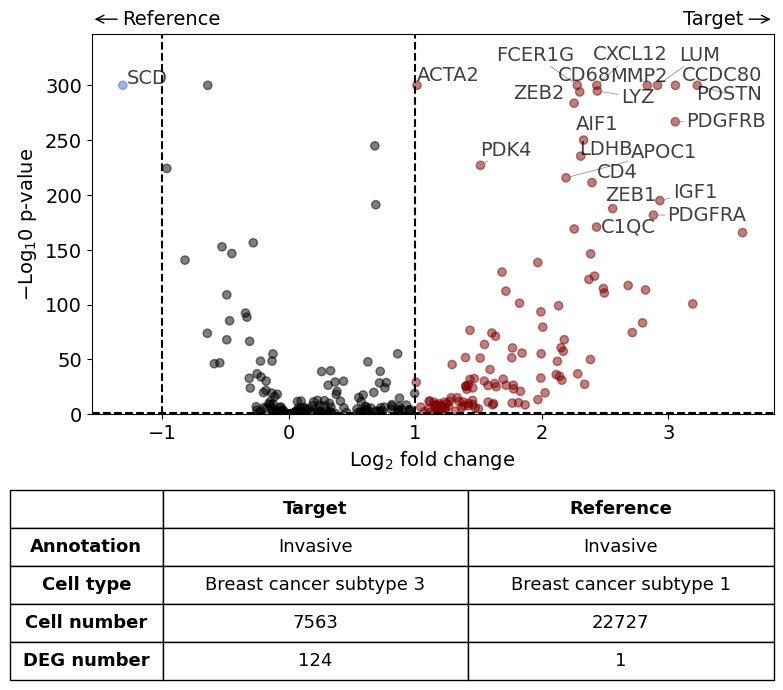
Subtype 1 and 3 in invasive tumor - 1 is in the center and 3 as outer budding layer. Also some individual tumor cells with subtype 3 found. What is the difference between the two subtypes?
DGE analysis within invasive Tumor annotation - subtype 3 vs. subtype 1
from insitupy import differential_gene_expression
differential_gene_expression(
    target=xd,
    target_annotation_tuple=("Katja", "Invasive"),
    ref_annotation_tuple="same",
    target_cell_type_tuple=("cell_type_dc_sub", "Breast cancer subtype 3"),
    ref_cell_type_tuple=("cell_type_dc_sub", "Breast cancer subtype 1"),
    exclude_ambiguous_assignments=True, # in this case we are sure that there
    savepath="figures/volcano_invasive_subtype3_vs_subtype1.pdf"
)
Calculate differentially expressed genes with Scanpy's `rank_genes_groups` using 't-test'.
Saving figure to file figures/volcano_invasive_subtype3_vs_subtype1.pdf
Saved.
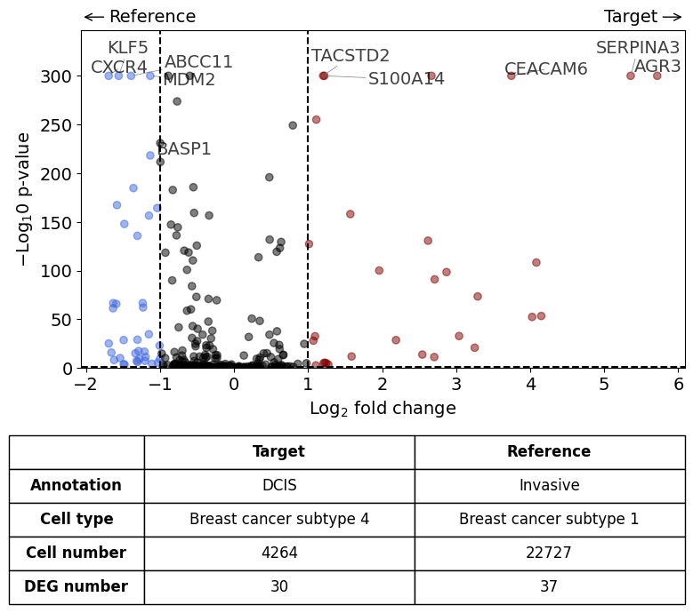
Comparison of DCIS vs invasive#
differential_gene_expression(
    target=xd,
    target_annotation_tuple=("Katja", "DCIS"),
    ref_annotation_tuple=("Katja", "Invasive"),
    target_cell_type_tuple=("cell_type_dc_sub", "Breast cancer subtype 4"),
    ref_cell_type_tuple=("cell_type_dc_sub", "Breast cancer subtype 1"),
    exclude_ambiguous_assignments=True, # in this case we are sure that there
    label_top_n=5,
    savepath="figures/volcano_subtype4_vs_subtype1.pdf"
)
Calculate differentially expressed genes with Scanpy's `rank_genes_groups` using 't-test'.
Saving figure to file figures/volcano_subtype4_vs_subtype1.pdf
Saved.
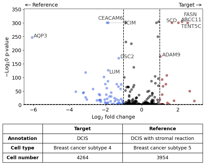
Comparison of DCIS vs DCIS with stromal reaction#
differential_gene_expression(
    target=xd,
    target_annotation_tuple=("Katja", "DCIS"),
    ref_annotation_tuple=("Katja", "DCIS with stromal reaction"),
    target_cell_type_tuple=("cell_type_dc_sub", "Breast cancer subtype 4"),
    ref_cell_type_tuple=("cell_type_dc_sub", "Breast cancer subtype 5"),
    exclude_ambiguous_assignments=True, # in this case we are sure that there
    label_top_n=5,
    savepath="figures/volcano_subtype4_vs_subtype5.pdf"
)
Calculate differentially expressed genes with Scanpy's `rank_genes_groups` using 't-test'.
Saving figure to file figures/volcano_subtype4_vs_subtype5.pdf
Saved.
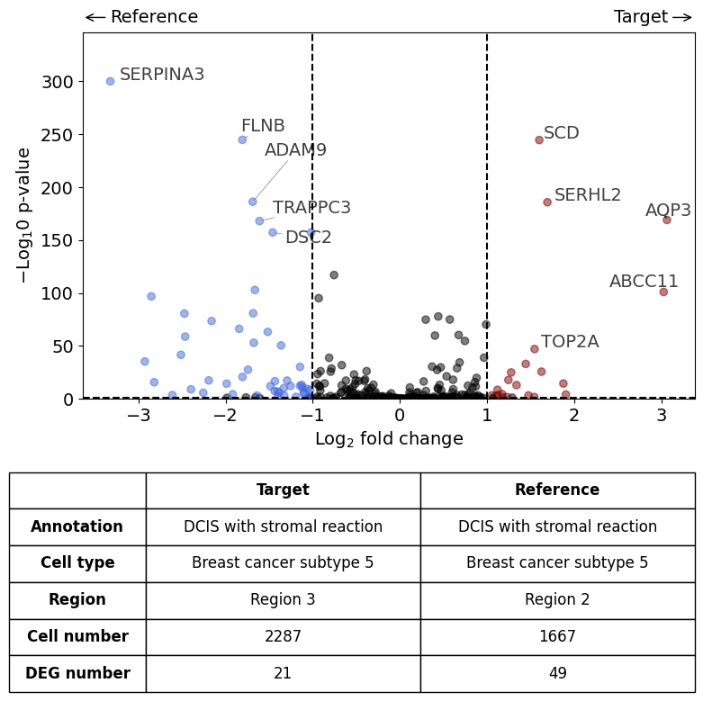
AQP3 expression higher in subtype 5 DCIS in Region 3 compared to subtype 5 DCIS in Region 2.#
differential_gene_expression(
    target=xd,
    target_annotation_tuple=("Katja", "DCIS with stromal reaction"),
    ref_annotation_tuple=("Katja", "DCIS with stromal reaction"),
    target_cell_type_tuple=("cell_type_dc_sub", "Breast cancer subtype 5"),
    ref_cell_type_tuple="same",
    target_region_tuple=("Katja", "Region 3"),
    ref_region_tuple=("Katja", "Region 2"),
    exclude_ambiguous_assignments=True, # in this case we are sure that there
    label_top_n=5,
    savepath="figures/volcano_stromalDCIS_region3_vs_region2.pdf"
)
Calculate differentially expressed genes with Scanpy's `rank_genes_groups` using 't-test'.
Saving figure to file figures/volcano_stromalDCIS_region3_vs_region2.pdf
Saved.
results = differential_gene_expression(
    target=xd,
    target_annotation_tuple=("Katja", "DCIS with stromal reaction"),
    ref_annotation_tuple=("Katja", "DCIS with stromal reaction"),
    target_cell_type_tuple=("cell_type_dc_sub", "Breast cancer subtype 5"),
    ref_cell_type_tuple="same",
    target_region_tuple=("Katja", "Region 3"),
    ref_region_tuple=("Katja", "Region 2"),
    exclude_ambiguous_assignments=True, # in this case we are sure that there
    label_top_n=5,
    return_results=True,
    savepath="figures/volcano_stromalDCIS_region3_vs_region2.pdf"
)
Calculate differentially expressed genes with Scanpy's `rank_genes_groups` using 't-test'.
Saving figure to file figures/volcano_stromalDCIS_region3_vs_region2.pdf
Saved.
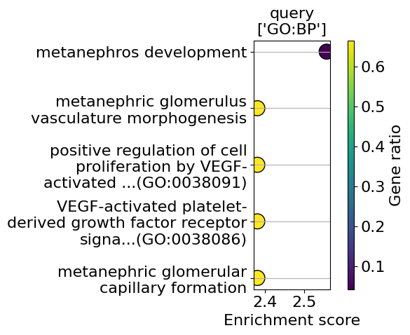
GO term enrichment analysis#
from insitupy.utils.go import GOEnrichment, get_up_down_genes
df = results["results"]
genes_up, genes_down = get_up_down_genes(df, pval_threshold=0.05, logfold_threshold=1)
genes_up
['SCD',
 'SERHL2',
 'AQP3',
 'ABCC11',
 'TOP2A',
 'CXCR4',
 'MKI67',
 'CENPF',
 'MZB1',
 'RAPGEF3',
 'CD68',
 'FCER1G',
 'HAVCR2',
 'NCAM1',
 'SOX18',
 'CCL5',
 'EGFL7',
 'SELL',
 'LY86',
 'TPSAB1',
 'RAMP2']
go = GOEnrichment()
go.gprofiler(target_genes=genes_up, key_added='up',
             top_n=20, organism="hsapiens", return_df=False)
go.gprofiler(target_genes=genes_down, key_added='down',
             top_n=20, organism="hsapiens", return_df=False)
go
GOEnrichment analyses performed:
  gprofiler:
    - up
    - down
enrichment = go.results["gprofiler"]["down"]
enrichment.head()
| source | native | name | p_value | significant | description | term_size | query_size | intersection_size | effective_domain_size | precision | Gene ratio | query | parents | intersections | evidences | Enrichment score | ||
|---|---|---|---|---|---|---|---|---|---|---|---|---|---|---|---|---|---|---|
| query | 0 | KEGG | KEGG:05215 | Prostate cancer | 0.000577 | True | Prostate cancer | 97 | 13 | 4 | 8484 | 0.307692 | 0.041237 | query_1 | [KEGG:00000] | [TCF7, ZEB1, PDGFRB, PDGFRA] | [[KEGG], [KEGG], [KEGG], [KEGG]] | 3.238647 |
| 1 | MIRNA | MIRNA:mmu-miR-200c-3p | mmu-miR-200c-3p | 0.000645 | True | mmu-miR-200c-3p | 2 | 18 | 2 | 14822 | 0.111111 | 1.000000 | query_1 | [MIRNA:000000] | [ZEB1, ZEB2] | [[MIRNA], [MIRNA]] | 3.190517 | |
| 2 | MIRNA | MIRNA:mmu-miR-200b-3p | mmu-miR-200b-3p | 0.000645 | True | mmu-miR-200b-3p | 2 | 18 | 2 | 14822 | 0.111111 | 1.000000 | query_1 | [MIRNA:000000] | [ZEB1, ZEB2] | [[MIRNA], [MIRNA]] | 3.190517 | |
| 3 | MIRNA | MIRNA:mmu-miR-200a-3p | mmu-miR-200a-3p | 0.000645 | True | mmu-miR-200a-3p | 2 | 18 | 2 | 14822 | 0.111111 | 1.000000 | query_1 | [MIRNA:000000] | [ZEB1, ZEB2] | [[MIRNA], [MIRNA]] | 3.190517 | |
| 4 | GO:MF | GO:0005017 | platelet-derived growth factor receptor activity | 0.000669 | True | "Combining with platelet-derived growth factor... | 3 | 19 | 2 | 20196 | 0.105263 | 0.666667 | query_1 | [GO:0004714] | [PDGFRB, PDGFRA] | [[IDA, IMP, IBA, TAS, IEA], [IDA, IMP, IBA, IEA]] | 3.174794 |
from insitupy.plotting.go import go_plot
go_plot(enrichment=enrichment,
        style='dot',
        libraries='GO:BP',
        max_to_plot=5,
        figsize=(6,5),
        savepath="figures/go_stromalDCIS_region3_vs_region2.pdf"
        )
Saving figure to file figures/go_stromalDCIS_region3_vs_region2.pdf
Saved.
Visualize data and save the colorlegends for publication#
xd.show()
xd.save_current_colorlegend("figures/colorlegend_SERPINA3.pdf")
Figure saved as figures/colorlegend_SERPINA3.pdf