Differential gene expression analysis for publication Figure 4#
## The following code ensures that all functions and init files are reloaded before executions.
%load_ext autoreload
%autoreload 2
from pathlib import Path
from insitupy import InSituData, CACHE
from insitupy.plotting import cellular_composition
import warnings
warnings.simplefilter(action='ignore', category=FutureWarning)
Load Xenium data into InSituData object#
Now the Xenium data can be parsed by providing the data path to the InSituPy project folder.
insitupy_project = Path(CACHE / "out/demo_insitupy_project")
xd = InSituData.read(insitupy_project)
xd.load_all()
xd.import_annotations(
    files=r"../../demo_data/demo_annotations/breast_cancer_annotations_publ.geojson",
    keys="Janesick",
    scale_factor=0.2125
)
xd.import_annotations(
    files=r"../../demo_data/demo_annotations/breast_cancer_annotations_Katja.geojson",
    keys="Katja",
    scale_factor=0.2125
)
xd.import_regions(
    files=r"../../demo_data/demo_annotations/breast_cancer_regions_Katja.geojson",
    keys="Katja",
    scale_factor=0.2125
)
xd
InSituData
Method:		Xenium
Slide ID:	0001879
Sample ID:	Replicate 1
Path:		C:\Users\ge37voy\.cache\InSituPy\out\demo_insitupy_project

    ➤ images
       CD20:	(25778, 35416)
       HE:	(25778, 35416, 3)
       HER2:	(25778, 35416)
       nuclei:	(25778, 35416)
    ➤ cells
       MultiCellData with main layer 'main'
           matrix
               AnnData object with n_obs × n_vars = 156447 × 297
               obs: 'transcript_counts', 'control_probe_counts', 'control_codeword_counts', 'total_counts', 'cell_area', 'nucleus_area', 'n_genes_by_counts', 'n_genes', 'leiden', 'cell_type_dc', 'cell_type_dc_sub', 'cell_type_tacco', 'cell_type_publ_x', 'cell_type_publ_y', 'cell_type_dc_sub_final', 'cell_type_publ'
               var: 'gene_ids', 'feature_types', 'genome', 'n_cells_by_counts', 'mean_counts', 'pct_dropout_by_counts', 'total_counts', 'n_cells'
               uns: 'cell_type_dc_colors', 'cell_type_dc_sub', 'cell_type_dc_sub_colors', 'cell_type_dc_sub_final_colors', 'cell_type_publ_colors', 'cell_type_tacco_colors', 'counts_location', 'leiden', 'leiden_colors', 'log1p', 'neighbors', 'pca', 'umap'
               obsm: 'OT', 'X_pca', 'X_umap', 'annotations', 'ora_estimate', 'ora_pvals', 'regions', 'spatial'
               varm: 'OT', 'PCs'
               layers: 'counts', 'norm_counts'
               obsp: 'connectivities', 'distances'
           boundaries
               BoundariesData object with 2 entries:
                   cells
                   nuclei
    ➤ transcripts
       DataFrame with shape <dask_expr.expr.Scalar: expr=ReadParquetFSSpec(77070fb).size() // 8, dtype=int64> x 8
    ➤ annotations
       TestKey:	5 annotations, 2 classes ('TestClass', 'test') ✔
       demo:	28 annotations, 2 classes ('Stroma', 'Tumor cells') ✔
       demo2:	5 annotations, 3 classes ('Negative', 'Other', 'Positive') ✔
       demo3:	7 annotations, 5 classes ('Immune cells', 'Necrosis', 'Stroma', 'Tumor', 'unclassified') ✔
       Demo:	28 annotations, 2 classes ('Stroma', 'Tumor cells') ✔
       Janesick:	18 annotations, 3 classes ('DCIS #1', 'DCIS #2', 'Invasive')
       Katja:	18 annotations, 4 classes ('DCIS', 'DCIS intermediate', 'DCIS with stromal reaction', 'Invasive') ✔
    ➤ regions
       demo_regions:	3 regions, 3 classes ('Region1', 'Region2', 'Region3') ✔
       TMA:	6 regions, 6 classes ('A-1', 'A-2', 'A-3', 'B-1', 'B-2', 'B-3') ✔
       Demo:	3 regions, 3 classes ('Region 1', 'Region 2', 'Region 3') ✔
       Katja:	4 regions, 4 classes ('Region 1', 'Region 2', 'Region 3', 'Region 4') ✔
xd.show()
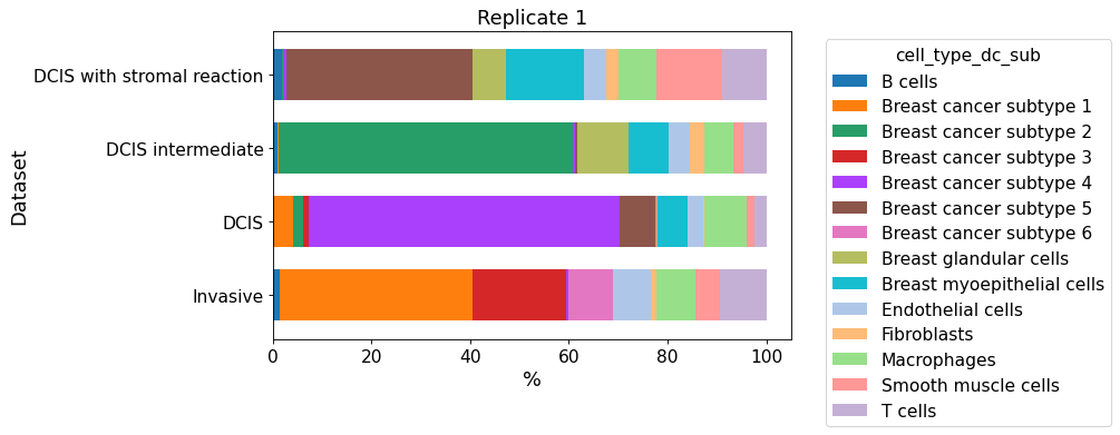
cellular_composition(
    data=xd, cell_type_col="cell_type_dc_sub",
    geom_key="Katja", modality="annotations", #max_cols=3,
    max_cols=1,
    plot_type="barh",
    savepath="figures/cell_composition_barh_annotations_Katja.pdf"
)
Since only one dataset is given, all regions are plotted into one figure.
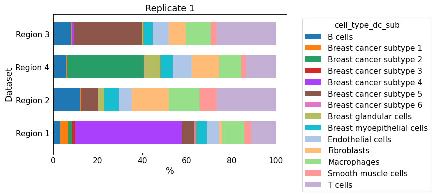
cellular_composition(
    data=xd, cell_type_col="cell_type_dc_sub",
    geom_key="Katja", modality="regions", #max_cols=3,
    max_cols=1,
    plot_type="barh",
    savepath="figures/cell_composition_barh_regions_Katja.pdf"
)
Since only one dataset is given, all regions are plotted into one figure.
xd.save()
Saving to existing path: C:\Users\ge37voy\.cache\InSituPy\out\demo_insitupy_project
Updating project in C:\Users\ge37voy\.cache\InSituPy\out\demo_insitupy_project
	Updating cells...
	Updating annotations...
	Updating regions...
Saved.
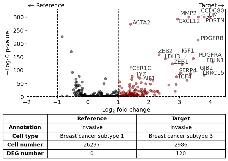
Next steps for DGE analysis#
Subtype 1 and 3 in invasive tumor - 1 is in the center and 3 as outer budding layer. Also some individual tumor cells with subtype 3 found. What is the difference between the two subtypes?
DGE analysis within invasive Tumor annotation - subtype 3 vs. subtype 1
from insitupy.tools import differential_gene_expression
xd.show()
differential_gene_expression(
    target=xd,
    target_annotation_tuple=("Katja", "Invasive"),
    ref_annotation_tuple="same",
    target_cell_type_tuple=("cell_type_dc_sub_final", "Breast cancer subtype 3"),
    ref_cell_type_tuple=("cell_type_dc_sub_final", "Breast cancer subtype 1"),
    exclude_ambiguous_assignments=True, # in this case we are sure that there
    #savepath="figures/volcano_invasive_subtype3_vs_subtype1.pdf"
)
Calculate differentially expressed genes with Scanpy's `rank_genes_groups` using 't-test'.
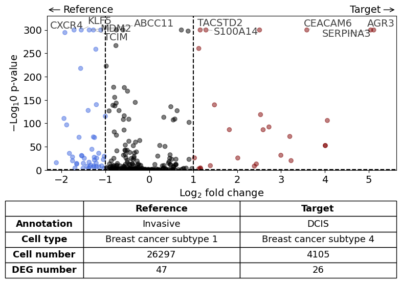
Comparison of DCIS vs invasive#
differential_gene_expression(
    target=xd,
    target_annotation_tuple=("Katja", "DCIS"),
    ref_annotation_tuple=("Katja", "Invasive"),
    target_cell_type_tuple=("cell_type_dc_sub_final", "Breast cancer subtype 4"),
    ref_cell_type_tuple=("cell_type_dc_sub_final", "Breast cancer subtype 1"),
    exclude_ambiguous_assignments=True, # in this case we are sure that there
    label_top_n=5,
    savepath="figures/volcano_subtype4_vs_subtype1.pdf"
)
Calculate differentially expressed genes with Scanpy's `rank_genes_groups` using 't-test'.
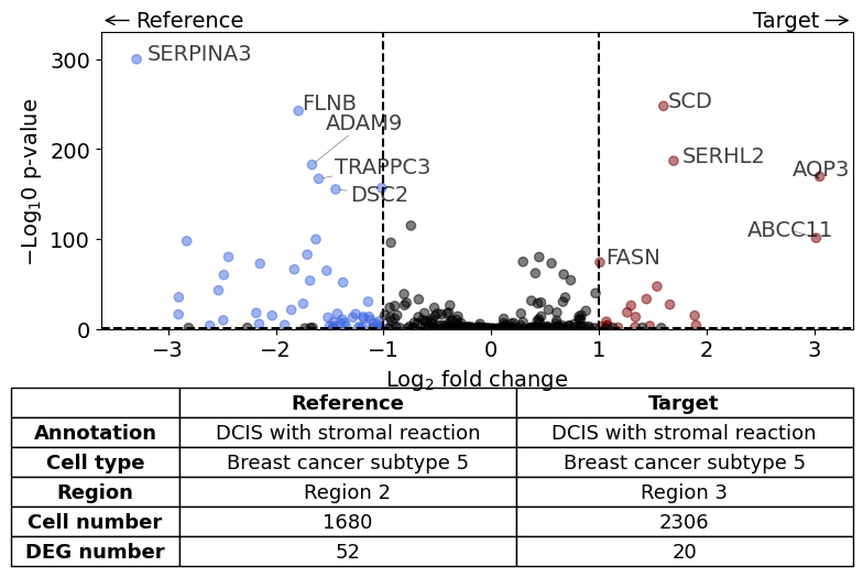
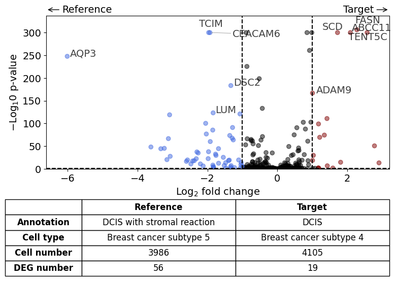
Comparison of DCIS vs DCIS with stromal reaction#
differential_gene_expression(
    target=xd,
    target_annotation_tuple=("Katja", "DCIS"),
    ref_annotation_tuple=("Katja", "DCIS with stromal reaction"),
    target_cell_type_tuple=("cell_type_dc_sub_final", "Breast cancer subtype 4"),
    ref_cell_type_tuple=("cell_type_dc_sub_final", "Breast cancer subtype 5"),
    exclude_ambiguous_assignments=True, # in this case we are sure that there
    label_top_n=5,
    savepath="figures/volcano_subtype4_vs_subtype5.pdf"
)
Calculate differentially expressed genes with Scanpy's `rank_genes_groups` using 't-test'.
AQP3 expression higher in subtype 5 DCIS in Region 3 compared to subtype 5 DCIS in Region 2.#
differential_gene_expression(
    target=xd,
    target_annotation_tuple=("Katja", "DCIS with stromal reaction"),
    ref_annotation_tuple=("Katja", "DCIS with stromal reaction"),
    target_cell_type_tuple=("cell_type_dc_sub_final", "Breast cancer subtype 5"),
    ref_cell_type_tuple="same",
    target_region_tuple=("Katja", "Region 3"),
    ref_region_tuple=("Katja", "Region 2"),
    exclude_ambiguous_assignments=True, # in this case we are sure that there
    label_top_n=5,
    savepath="figures/volcano_stromalDCIS_region3_vs_region2.pdf"
)
Calculate differentially expressed genes with Scanpy's `rank_genes_groups` using 't-test'.