Data preprocessing and analysis

## The following code ensures that all functions and init files are reloaded before executions.
%load_ext autoreload
%autoreload 2

from pathlib import Path
import scanpy as sc
from insitupy import InSituData, CACHE

Load Xenium data into InSituData object

Now the Xenium data can be parsed by providing the data path to the InSituPy project folder.

# prepare paths
data_dir = Path(CACHE / "out/demo_insitupy_project") # directory of xenium data
xd = InSituData.read(data_dir)

xd

InSituData
Method:		Xenium
Slide ID:	0001879
Sample ID:	Replicate 1
Path:		C:\Users\ge37voy\.cache\InSituPy\out\demo_insitupy_project


No modalities loaded.

# read all data modalities at once
xd.load_all()

# alternatively, it is also possible to read each modality separately
# xd.load_cells()
# xd.load_images()
# xd.load_transcripts()
# xd.read_annotations()

Note: That the annotations and regions modalities are not found here is expected. Annotations are added in a later step.

xd

InSituData
Method:		Xenium
Slide ID:	0001879
Sample ID:	Replicate 1
Path:		C:\Users\ge37voy\.cache\InSituPy\out\demo_insitupy_project

    ➤ images
       CD20:	(25778, 35416)
       HE:	(25778, 35416, 3)
       HER2:	(25778, 35416)
       nuclei:	(25778, 35416)
    ➤ cells
       MultiCellData with main layer 'main'
           matrix
               AnnData object with n_obs × n_vars = 167780 × 313
               obs: 'transcript_counts', 'control_probe_counts', 'control_codeword_counts', 'total_counts', 'cell_area', 'nucleus_area'
               var: 'gene_ids', 'feature_types', 'genome'
               obsm: 'spatial'
           boundaries
               BoundariesData object with 2 entries:
                   cells
                   nuclei
    ➤ transcripts
       DataFrame with shape <dask_expr.expr.Scalar: expr=ReadParquetFSSpec(c96cbd3).size() // 8, dtype=int64> x 8

Explore data in interactive napari viewer

Example image of the viewer:

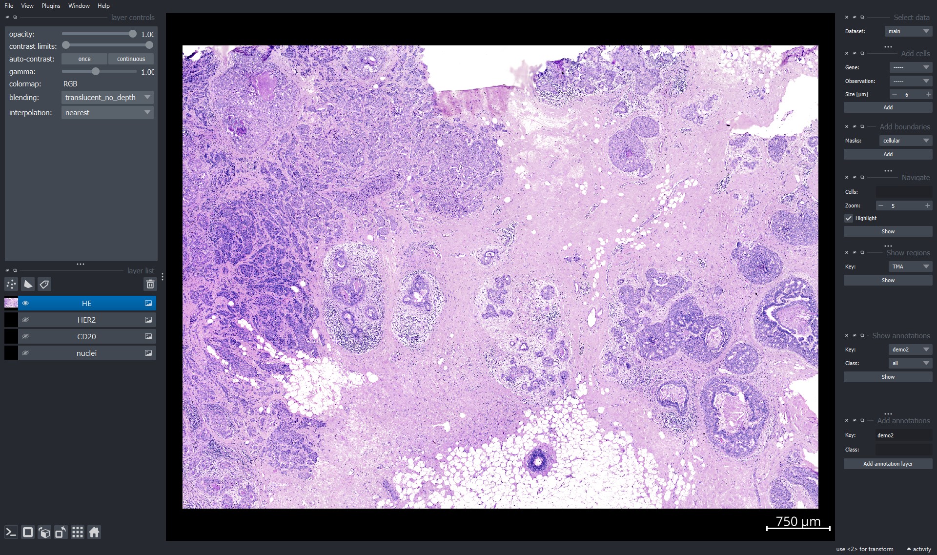
For detailed documentation on the functionalities of napari see the official documentation here.

xd.show()

Explore gene expression using napari viewer

Use the "Add cells" widget to explore the single-cell transcriptomic data.

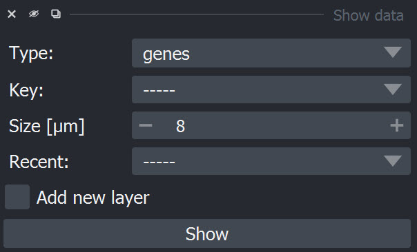
Genes can be selected from the dropdown window by scrolling or by clicking into the window and typing the name of the item:

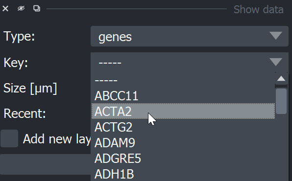
After selection of an item it can be added using the "Add" button. The data is added as point layer to the napari viewer.

Perform preprocessing steps

InSituPy also includes basic preprocessing functions to normalize the transcriptomic data and perform dimensionality reduction. For normalization, the ScanPy function sc.pp.normalize_total() is used. Data transformation can be either done using logarithmic transformation or square root transformation as suggested here.

For a general introduction into preprocessing steps in single-cell transcriptomics analysis, the single-cell best practices book is a great ressource.

Calculate QC metrics

Now we use the function calculate_qc_metrics to calculate the QC metrics, which we will afterwards use to filter the data and remove low quality cells. The function takes either an InSituData or InSituExperiment object. If you have multiple cell layers, it is important to specify the correct cells_layer.

from insitupy.preprocessing import calculate_qc_metrics

calculate_qc_metrics(xd, cells_layer="main", percent_top=None, log1p=False)

Filtering

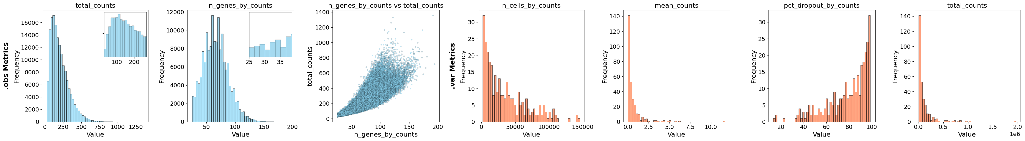
In our experience the QC metrices can vary a lot between different samples. Therefore, it is important to explore every dataset separately before making decisions on filtering thresholds. Also, it can be beneficial to try to split the dataset before filtering into different cell lineages (e.g. epithelial vs. non-epithelial) and use different thresholds per lineage, since even within cell types there can be large variations in the QC metrices. This can be especially the case for technologies like Xenium where a rather small gene panel is used and the transcript counts depend a lot on whether the panel contains marker genes of a certain cell type or not.

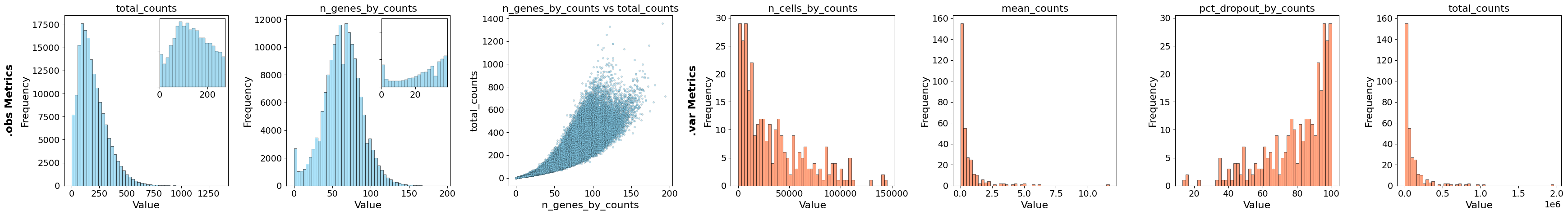
from insitupy.plotting import plot_qc_metrics

plot_qc_metrics(xd, show_inset=True)

For filtering there are different options, but in this case we chose to filter on two parameters: n_genes_by_counts and n_cell_by_counts. The first parameter filters out cells (.obs) in which only a very small number of genes were found and the second parameter filters out genes (.var) which were only found in a very small number of cells. As threshold we chose cells with less than 25 genes and genes which were found in less than 1% of the cells. Filtering of cells happens on the level of .cells.matrix. To synchronize the cells included in .cells.matrix and their boundaries in .cells.boundaries after the filtering, .sync is called within the filter_cells function.

from insitupy.preprocessing import filter_cells, filter_genes

filter_cells(xd, min_genes=25)

xd.cells.matrix

AnnData object with n_obs × n_vars = 157600 × 313
    obs: 'transcript_counts', 'control_probe_counts', 'control_codeword_counts', 'total_counts', 'cell_area', 'nucleus_area', 'n_genes_by_counts', 'n_genes'
    var: 'gene_ids', 'feature_types', 'genome', 'n_cells_by_counts', 'mean_counts', 'pct_dropout_by_counts', 'total_counts'
    obsm: 'spatial'

cell_number = xd.cells.matrix.shape[0]
cell_threshold = int(cell_number * 0.01)
print(f"Threshold for cells per gene: {cell_threshold}")

Threshold for cells per gene: 1576

filter_genes(xd, min_cells=cell_threshold)

xd.cells.matrix

AnnData object with n_obs × n_vars = 157600 × 297
    obs: 'transcript_counts', 'control_probe_counts', 'control_codeword_counts', 'total_counts', 'cell_area', 'nucleus_area', 'n_genes_by_counts', 'n_genes'
    var: 'gene_ids', 'feature_types', 'genome', 'n_cells_by_counts', 'mean_counts', 'pct_dropout_by_counts', 'total_counts', 'n_cells'
    obsm: 'spatial'

After the filter the QC metrices look as follows:

plot_qc_metrics(xd)

Normalization and transformation

Two transformation methods were suggested for transforming in situ sequencing data: log-transformation and square root-transformation. To test which one is better suited for the current dataset, the test_transformation function can be used.

from insitupy.plotting import test_transformations

test_transformations(
    xd, target_sum=250, scale=False
    )

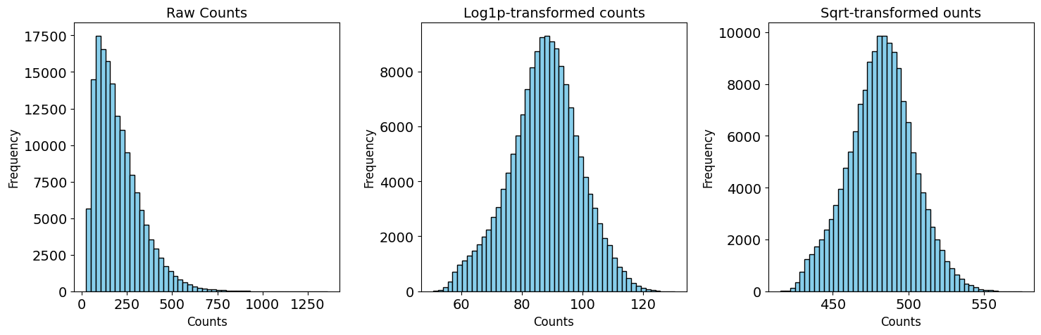
Here, we decided to continue with the log-transformation, which is also the most common approach.

from insitupy.preprocessing import normalize_and_transform

normalize_and_transform(
    data=xd,
    transformation_method="log1p",
    target_sum=250,
    scale=False,
    verbose=True
    )

Store raw counts in .layers['counts'].
Normalization with target sum 250.
Perform log1p-transformation.

Dimensionality reduction

Calculating the UMAP can take about 5-10 min due to the size of the dataset.

from insitupy.preprocessing import reduce_dimensions, cluster_cells

reduce_dimensions(
    data=xd,
    cells_layer="main",
    n_neighbors=15,
    n_pcs=None
    )

Calculate PCA...
Calculate neighbors...
Calculate umap...

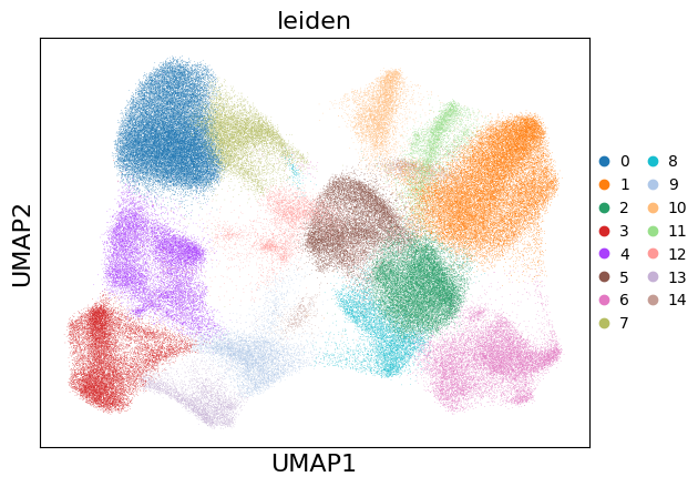
cluster_cells(
    data=xd,
    cells_layer="main", # or None to use the layer specified in .main_key
    method="leiden"
)

Show results using scanpy functions

sc.pl.umap(xd.cells.matrix, color=["leiden"])

# visualize data
xd.show()

Start viewer with list of selected genes

Alternatively to selecting genes inside the napari viewer, it is also possible to open the viewer directly including a list of genes.

xd.show(keys=["leiden", "ACTA2", "LYZ", "LUM"])

Genes can be displayed or hidden via the eye symbol:

Save results within InSituPy project

The processed data can be saved into a folder using the .saveas() function of InSituData.

The resulting folder has following structure (can vary depending on which modalities have been loaded before):

insitupy_project_folder
│   .ispy
│
├───cells
│   └───uid
│       │   .celldata
│       │
│       ├───boundaries
│       │       cellular.zarr.zip
│       │       nuclear.zarr.zip
│       │
│       └───matrix
│               matrix.h5ad
│
├───images
│       morphology_mip.zarr.zip
│       slide_id__sample_id__CD20__registered.zarr.zip
│       slide_id__sample_id__HER2__registered.zarr.zip
│       slide_id__sample_id__HE__registered.zarr.zip
│
└───transcripts
        transcripts.parquet

xd.save()

Saving to existing path: C:\Users\ge37voy\.cache\InSituPy\out\demo_insitupy_project
Updating project in C:\Users\ge37voy\.cache\InSituPy\out\demo_insitupy_project
	Updating cells...
Saved.

xd

InSituData
Method:		Xenium
Slide ID:	0001879
Sample ID:	Replicate 1
Path:		C:\Users\ge37voy\.cache\InSituPy\out\demo_insitupy_project

    ➤ images
       CD20:	(25778, 35416)
       HE:	(25778, 35416, 3)
       HER2:	(25778, 35416)
       nuclei:	(25778, 35416)
    ➤ cells
       MultiCellData with main layer 'main'
           matrix
               AnnData object with n_obs × n_vars = 157600 × 297
               obs: 'transcript_counts', 'control_probe_counts', 'control_codeword_counts', 'total_counts', 'cell_area', 'nucleus_area', 'n_genes_by_counts', 'n_genes', 'leiden'
               var: 'gene_ids', 'feature_types', 'genome', 'n_cells_by_counts', 'mean_counts', 'pct_dropout_by_counts', 'total_counts', 'n_cells'
               uns: 'leiden', 'leiden_colors', 'log1p', 'neighbors', 'pca', 'umap'
               obsm: 'X_pca', 'X_umap', 'spatial'
               varm: 'PCs'
               layers: 'counts', 'norm_counts'
               obsp: 'connectivities', 'distances'
           boundaries
               BoundariesData object with 2 entries:
                   cells
                   nuclei
    ➤ transcripts
       DataFrame with shape <dask_expr.expr.Scalar: expr=ReadParquetFSSpec(c96cbd3).size() // 8, dtype=int64> x 8

Experimental function: Version history of data

It is also possible to keep a version history of the “variable” data in InSituPy. As variable data InSituPy considers .cells, .annotations and .regions. By default keep_history=False, but if you want to keep the history, it is also possible to set keep_history=True as in the following example. Importantly, if you want to keep the history, it is important to always set keep_history=True. Otherwise the history gets deleted the next time you just use .save(). This behavior is not really optimal and we will try to find a solution for that in the future.

#xd.save(keep_history=True)