Pseudobulk Differential Gene Expression Analysis in InSituPy

This tutorial demonstrates how to perform pseudobulk differential gene expression (DGE) analysis using InSituPy. Pseudobulk analysis aggregates single-cell counts by sample and cell type, enabling statistical testing with established bulk RNA-seq methods.

When to use pseudobulk analysis:

• Comparing gene expression between experimental conditions

• Analyzing regional differences in spatial transcriptomics data

• When you have multiple biological replicates per condition

More information on why to use pseudobulking, can be found in this decoupler tutorial.

1. Setup and Data Loading

from insitupy._core.data import InSituData, CACHE
from insitupy import InSituExperiment
from insitupy.preprocessing import pseudobulk
from insitupy.tools import pseudobulk_dge
from insitupy.plotting import volcano, dual_foldchange_plot
from insitupy.dataclasses.results import DiffExprResults
import decoupler as dc
from pathlib import Path

Load Xenium Data

Load preprocessed Xenium data containing spatial transcriptomics information with cell segmentation and annotations.

# Update this path to your data location
data_path = Path(CACHE / "out/demo_insitupy_project")
xd = InSituData.read(data_path)
xd.load_all(skip="transcripts")  # Load all data except transcript coordinates
xd

InSituData
Method:		Xenium
Slide ID:	0001879
Sample ID:	Replicate 1
Path:		C:\Users\ge37voy\.cache\InSituPy\out\demo_insitupy_project

    ➤ images
       CD20:	(25778, 35416)
       HE:	(25778, 35416, 3)
       HER2:	(25778, 35416)
       nuclei:	(25778, 35416)
    ➤ cells
       MultiCellData with main layer 'main'
           matrix
               AnnData object with n_obs × n_vars = 156447 × 297
               obs: 'transcript_counts', 'control_probe_counts', 'control_codeword_counts', 'total_counts', 'cell_area', 'nucleus_area', 'n_genes_by_counts', 'n_genes', 'leiden', 'cell_type_dc', 'cell_type_dc_sub', 'cell_type_tacco', 'cell_type_publ_x', 'cell_type_publ_y', 'cell_type_dc_sub_final', 'cell_type_publ'
               var: 'gene_ids', 'feature_types', 'genome', 'n_cells_by_counts', 'mean_counts', 'pct_dropout_by_counts', 'total_counts', 'n_cells'
               uns: 'cell_type_dc_colors', 'cell_type_dc_sub', 'cell_type_dc_sub_colors', 'cell_type_dc_sub_final_colors', 'cell_type_publ_colors', 'cell_type_tacco_colors', 'counts_location', 'leiden', 'leiden_colors', 'log1p', 'neighbors', 'pca', 'umap'
               obsm: 'OT', 'X_pca', 'X_umap', 'annotations', 'ora_estimate', 'ora_pvals', 'regions', 'spatial'
               varm: 'OT', 'PCs'
               layers: 'counts', 'norm_counts'
               obsp: 'connectivities', 'distances'
           boundaries
               BoundariesData object with 2 entries:
                   cells
                   nuclei
    ➤ annotations
       TestKey:	5 annotations, 2 classes ('TestClass', 'test') ✔
       demo:	28 annotations, 2 classes ('Stroma', 'Tumor cells') ✔
       demo2:	5 annotations, 3 classes ('Negative', 'Other', 'Positive') ✔
       demo3:	7 annotations, 5 classes ('Immune cells', 'Necrosis', 'Stroma', 'Tumor', 'unclassified') ✔
       Demo:	28 annotations, 2 classes ('Stroma', 'Tumor cells') ✔
       Janesick:	18 annotations, 3 classes ('DCIS #1', 'DCIS #2', 'Invasive') 
       Katja:	18 annotations, 4 classes ('DCIS', 'DCIS intermediate', 'DCIS with stromal reaction', 'Invasive') ✔
    ➤ regions
       demo_regions:	3 regions, 3 classes ('Region1', 'Region2', 'Region3') ✔
       TMA:	6 regions, 6 classes ('A-1', 'A-2', 'A-3', 'B-1', 'B-2', 'B-3') ✔
       Demo:	3 regions, 3 classes ('Region 1', 'Region 2', 'Region 3') ✔
       Katja:	4 regions, 4 classes ('Region 1', 'Region 2', 'Region 3', 'Region 4') ✔

2. Create InSituExperiment from Regions

Since we do not actually have multiple samples in this dataset, we will create a dummy multi-sample TMA dataset in this step. For this, we will use InSituExperiments crop function based on regions resembling a TMA core layout.

exp = InSituExperiment.from_regions(
    data=xd,
    region_key="TMA"  # Column in annotations containing region IDs
)

A-1
A-2
A-3
B-1
B-2
B-3

exp

InSituExperiment with 6 samples:
           uid  CITAR slide_id    sample_id region_key region_name
0     63233d00  ++-++  0001879  Replicate 1        TMA         A-1
1     4954bee6  ++-++  0001879  Replicate 1        TMA         A-2
2     689152e7  ++-++  0001879  Replicate 1        TMA         A-3
3     ba169d36  ++-++  0001879  Replicate 1        TMA         B-1
4     b40447da  ++-++  0001879  Replicate 1        TMA         B-2
5     47c7fda7  ++-++  0001879  Replicate 1        TMA         B-3

3. Define Experimental Conditions

⚠️ Important: This tutorial uses dummy conditions for demonstration. In a real analysis, conditions should reflect meaningful biological groups (e.g., treatment vs. control, disease vs. healthy).

Add metadata specifying which condition each sample belongs to:

# Assign conditions: first 3 regions to condition A, last 3 to condition B
exp.add_metadata_column(
    column_name="condition",
    values=["A", "A", "A", "B", "B", "B"]
)

# Verify metadata structure
exp.metadata

You are accessing a copy of the metadata. Changes to this DataFrame will not affect the internal metadata. Use `add_metadata_column()` or `append_metadata()` to add new information to the metadata.

	uid	slide_id	sample_id	region_key	region_name	condition
0	f2c0a45e	0001879	Replicate 1	TMA	A-1	A
1	2ef07500	0001879	Replicate 1	TMA	A-2	A
2	ea568462	0001879	Replicate 1	TMA	A-3	A
3	3f73f030	0001879	Replicate 1	TMA	B-1	B
4	80235888	0001879	Replicate 1	TMA	B-2	B
5	13b4a354	0001879	Replicate 1	TMA	B-3	B

4. Generate Pseudobulk Data

Aggregate single-cell counts into pseudobulk samples. This creates one pseudobulk profile per (sample × cell type) combination.

Key parameters:

• celltype_col: Cell type annotation column to aggregate by

• counts_layer: Raw count matrix layer (use unnormalized counts)

• metadata_to_transfer: Experimental design variables to include

• calculate_neighbors: Determines whether or not to calculate the pseudobulk data of the neighboring cells.

For detailed information, see the decoupler pseudobulk documentation.

Generating pseudobulk of the target cells only

Using calculate_neighbors=False we can calculate the pseudobulk profiles of the target cells only.

pdata = pseudobulk(
    exp=exp,
    celltype_col='cell_type_dc_sub_final',
    cells_layer='main',
    counts_layer='counts',  # Use raw counts, not normalized
    calculate_neighbors=False,
    metadata_to_transfer="condition"
)

# Inspect pseudobulk structure
pdata

AnnData object with n_obs × n_vars = 73 × 297
    obs: 'uid', 'cell_type_dc_sub_final', 'psbulk_cells', 'psbulk_counts', 'condition', 'obs_type'
    uns: 'pseudobulk_settings'
    layers: 'psbulk_props'

# View sample metadata
pdata.obs

	uid	cell_type_dc_sub_final	psbulk_cells	psbulk_counts	condition	obs_type
f2c0a45e_B cells	f2c0a45e	B cells	86.0	12128.0	A	cells
f2c0a45e_Breast cancer subtype 1	f2c0a45e	Breast cancer subtype 1	568.0	132467.0	A	cells
f2c0a45e_Breast cancer subtype 2	f2c0a45e	Breast cancer subtype 2	76.0	10725.0	A	cells
f2c0a45e_Breast cancer subtype 3	f2c0a45e	Breast cancer subtype 3	50.0	13919.0	A	cells
f2c0a45e_Breast cancer subtype 4	f2c0a45e	Breast cancer subtype 4	2379.0	528355.0	A	cells
...	...	...	...	...	...	...
13b4a354_Endothelial cells	13b4a354	Endothelial cells	218.0	38530.0	B	cells
13b4a354_Macrophages	13b4a354	Macrophages	459.0	84097.0	B	cells
13b4a354_Smooth muscle cells	13b4a354	Smooth muscle cells	81.0	12949.0	B	cells
13b4a354_Stromal cells	13b4a354	Stromal cells	633.0	146404.0	B	cells
13b4a354_T cells	13b4a354	T cells	252.0	34913.0	B	cells

73 rows × 6 columns

Taking Neighborhood Effects into account

Imaging-based spatial transcriptomics methods (e.g., Xenium, MERSCOPE) assign transcripts to cells through segmentation, a process prone to boundary errors. Misassigned transcripts can contaminate cell expression profiles, particularly when neighboring cells have distinct expression patterns.

To assess potential neighborhood contamination, set calculate_neighbors=True in the pseudobulk function. This returns a second pseudobulk dataset (pdata_nb) aggregating gene expression counts of cells that are within a certain radius (neighbors_radius) of either the target or the reference cells. This enables comparison between target cells and reference cells and their respective microenvironment to identify spillover effects.

pdata, pdata_nb = pseudobulk(
    exp=exp,
    celltype_col='cell_type_dc_sub_final',
    cells_layer='main',
    counts_layer='counts',  # Use raw counts, not normalized
    calculate_neighbors=True,
    neighbors_radius=20,
    metadata_to_transfer="condition"
)

pdata

AnnData object with n_obs × n_vars = 73 × 297
    obs: 'uid', 'cell_type_dc_sub_final', 'psbulk_cells', 'psbulk_counts', 'condition', 'obs_type'
    uns: 'pseudobulk_settings'
    layers: 'psbulk_props'

pdata_nb

AnnData object with n_obs × n_vars = 73 × 297
    obs: 'uid', 'psbulk_cells', 'psbulk_counts', 'cell_type_dc_sub_final', 'condition', 'obs_type'
    uns: 'pseudobulk_settings'
    layers: 'psbulk_props'

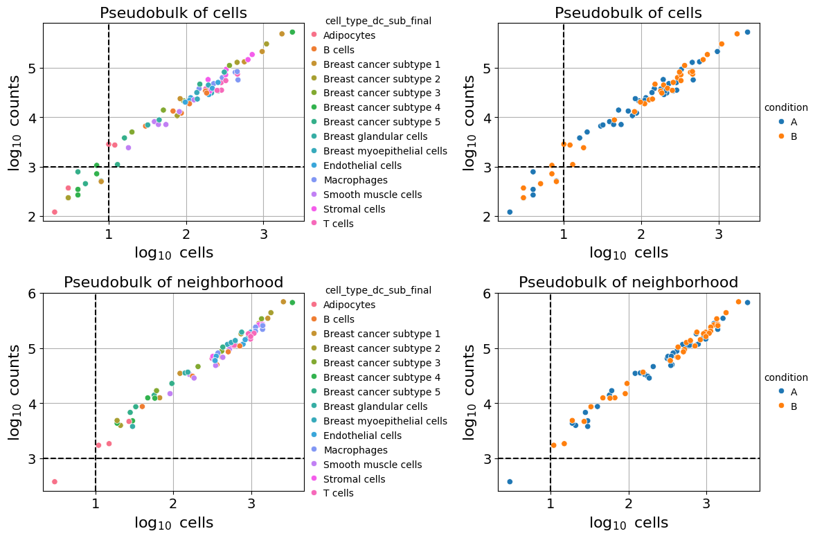
5. Differential Expression Analysis

Quality Control and Filtering

Filter low-quality pseudobulk samples based on cell count and total reads. This ensures sufficient data for statistical testing.

Filtering criteria:

• min_cells: Minimum cells per pseudobulk sample (default: 10)

• min_counts: Minimum total counts per pseudobulk sample (default: 1000)

Samples failing these thresholds are excluded from analysis. Whether or not to show the QC plots can be determined with the plot_qc argument.

Setting up differential gene expression analysis

Perform DE testing using PyDESeq2 with a Wald test. This identifies genes with significant expression changes between conditions.

Analysis setup:

• dge_setup: [“condition_column”, “reference_group”, “comparison_group”]

• Tests are performed separately for each cell type

• Uses DESeq2 normalization and dispersion estimation

• Wald test statistic: tests H₀: log2(fold change) = 0

# Define comparison: condition A vs B for Endothelial cells
dge_setup = ["condition", "A", "B"]  # [column, reference, comparison]
celltype_col = "cell_type_dc_sub_final"
celltype = "Endothelial cells"

# Run differential expression analysis
dge_results = pseudobulk_dge(
    pdata=pdata,
    pdata_nb=pdata_nb,
    dge_setup=dge_setup,
    celltype_col=celltype_col,
    celltype=celltype,
    plot_qc=True,  # Display QC plots
    min_cells=10,
    min_counts=1000
)

Sample filtering QC:
Filtered pseudobulk samples: 13 removed, 60 remaining (out of 73 total).
Filtered pseudobulk samples: 1 removed, 72 remaining (out of 73 total).
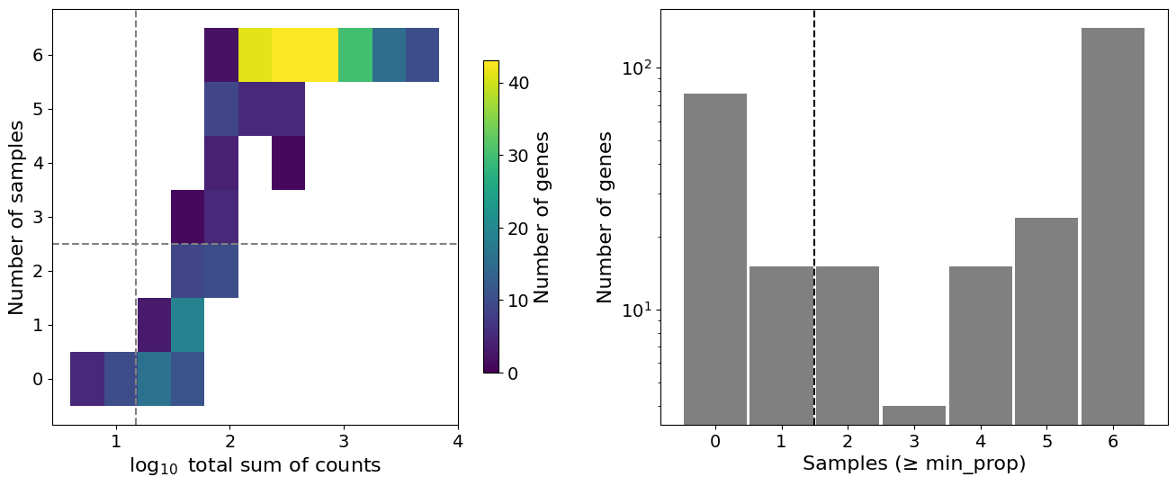
Feature filtering QC:
Filtered features: 94 removed, 203 remaining (out of 297 total).

Inspect Results

Results are returned as DiffExprResults object and contain, depending on the choice of calculate_neighbors following attributes:

• .main: Includes the DGE results of target vs. reference

• With calculate_neighbors=True:

  • .target_neighborhood: DGE results of target cells vs. their neighboring cells

  • .ref_neighborhood: DGE results of reference cells vs. their neighboring cells

Each attribute is a pandas DataFrame with following columns:

• log2foldchange: Effect size (positive = upregulated in comparison group)

• pvalue: Unadjusted p-value from Wald test

• padj: Benjamini-Hochberg adjusted p-value (FDR)

• baseMean: Mean normalized expression across all samples

• lfcSE: Standard error of log2 fold change estimate

dge_results

<DiffExprResults main=203 genes, neighbors=True>

dge_results.target_neighborhood

	baseMean	log2foldchange	lfcSE	stat	pvalue	padj
TCEAL7	15.718131	0.029246	0.706394	0.041402	0.966975	0.983001
SERPINA3	169.857821	-1.068293	0.804259	-1.328294	0.184081	0.336653
OXTR	25.867383	-0.578630	1.008900	-0.573525	0.566289	0.699190
VOPP1	258.095754	0.201572	0.280058	0.719751	0.471678	0.629939
SLAMF7	42.654832	-1.381457	0.806041	-1.713880	0.086551	0.186913
...	...	...	...	...	...	...
BASP1	167.276937	-0.083483	0.456860	-0.182731	0.855009	0.936253
CCND1	1107.843556	0.006432	0.343226	0.018740	0.985048	0.994850
PIM1	54.493571	0.315380	0.436514	0.722497	0.469989	0.629939
GPR183	51.245005	-1.105145	0.489737	-2.256608	0.024033	0.067258
RAB30	56.988037	0.396197	0.402177	0.985131	0.324559	0.495380

203 rows × 6 columns

dge_results.ref_neighborhood

	baseMean	log2foldchange	lfcSE	stat	pvalue	padj
TCEAL7	38.239049	0.112318	0.627172	0.179087	0.857870	0.984517
SERPINA3	369.253368	-0.591137	0.813881	-0.726319	0.467643	0.713772
OXTR	32.981467	0.542059	0.456635	1.187071	0.235199	0.467345
VOPP1	336.178636	0.022524	0.231812	0.097165	0.922596	0.984517
SLAMF7	84.889624	-1.270426	0.481079	-2.640787	0.008271	0.039049
...	...	...	...	...	...	...
BASP1	256.730384	-0.480564	0.415231	-1.157339	0.247134	0.474292
CCND1	1234.364714	0.035665	0.370002	0.096392	0.923209	0.984517
PIM1	105.199901	-0.241432	0.430210	-0.561196	0.574664	0.815782
GPR183	87.687705	-1.171416	0.328587	-3.565012	0.000364	0.002736
RAB30	86.900815	-0.036018	0.382071	-0.094269	0.924895	0.984517

203 rows × 6 columns

# View top differentially expressed genes
dge_results.main.sort_values('log2foldchange', ascending=False).head(10)

	baseMean	log2foldchange	lfcSE	stat	pvalue	padj
STC1	42.618256	1.552160	0.619546	2.505320	0.012234	0.98202
TOP2A	53.314037	0.983508	0.758607	1.296467	0.194815	0.98202
CENPF	26.694345	0.822907	0.779076	1.056259	0.290850	0.98202
EPCAM	101.539657	0.719454	0.580242	1.239919	0.215005	0.98202
MLPH	59.747752	0.642235	0.739827	0.868087	0.385347	0.98202
S100A14	55.779857	0.604616	0.429980	1.406149	0.159680	0.98202
AIF1	80.345539	0.549303	0.279633	1.964370	0.049487	0.98202
MYH11	40.690712	0.536262	0.945131	0.567395	0.570446	0.98202
ANKRD30A	143.662662	0.528604	0.531122	0.995258	0.319611	0.98202
EIF4EBP1	32.833096	0.508238	0.494774	1.027214	0.304320	0.98202

6. Save and Load Results

Save results to disk for later analysis or sharing.

# Save results
output_dir = "out/pseudobulk_dge/"
dge_results.save(output_dir, overwrite=True)

Warning: Overwriting existing directory 'out\pseudobulk_dge'.

# Load previously saved results
dr = DiffExprResults.read(output_dir)

7. Visualization

Visualize differential expression results to identify significant genes.

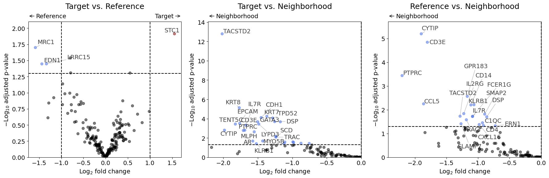
Volcano Plot

Shows significance (y-axis) vs. effect size (x-axis). Points in the upper corners represent genes with large fold changes and high significance. Since none of the genes in this dummy experiment show a significant result in the adjusted p-values, we will plot for demonstration purposes the "pvalue" instead of "padj" (which is the default).

volcano(dr, pval_col="pvalue")

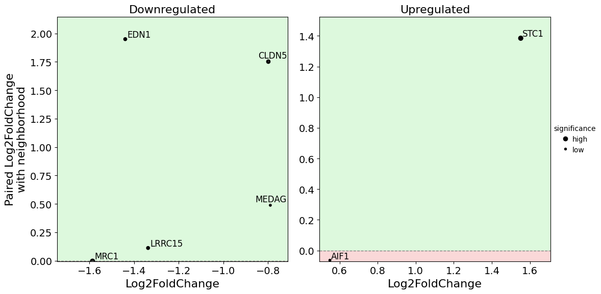
Dual Fold Change Plot

Compares fold changes across two comparisons or displays expression patterns. Useful for identifying genes with consistent changes across multiple contrasts.

dual_foldchange_plot(
    dr,
    pval_col="pvalue",
    show_nonsignificant=False
    )