Plot colorlegends for publication

## The following code ensures that all functions and init files are reloaded before executions.
%load_ext autoreload
%autoreload 2

# import packages
from pathlib import Path
from insitupy import InSituData, CACHE
import warnings
warnings.simplefilter(action='ignore', category=FutureWarning)

Load Xenium data into InSituData object

Now the Xenium data can be parsed by providing the data path to the InSituPy project folder.

insitupy_project = Path(CACHE / "out/demo_insitupy_project")

xd = InSituData.read(insitupy_project)
xd.load_all()

xd

InSituData
Method:		Xenium
Slide ID:	0001879
Sample ID:	Replicate 1
Path:		C:\Users\ge37voy\.cache\InSituPy\out\demo_insitupy_project
Metadata file:	.ispy
    ➤ images
       nuclei:	(25778, 35416)
       CD20:	(25778, 35416)
       HER2:	(25778, 35416)
       HE:	(25778, 35416, 3)
    ➤ cells
       MultiCellData with main layer 'main'
           matrix
               AnnData object with n_obs × n_vars = 156447 × 297
               obs: 'transcript_counts', 'control_probe_counts', 'control_codeword_counts', 'total_counts', 'cell_area', 'nucleus_area', 'n_genes_by_counts', 'n_genes', 'leiden', 'cell_type_dc', 'cell_type_dc_sub', 'cell_type_tacco', 'cell_type_publ'
               var: 'gene_ids', 'feature_types', 'genome', 'n_cells_by_counts', 'mean_counts', 'pct_dropout_by_counts', 'total_counts', 'n_cells'
               uns: 'cell_type_dc_colors', 'cell_type_dc_sub', 'cell_type_dc_sub_colors', 'cell_type_publ_colors', 'cell_type_tacco_colors', 'counts_location', 'leiden', 'leiden_colors', 'log1p', 'neighbors', 'pca', 'umap'
               obsm: 'OT', 'X_pca', 'X_umap', 'annotations', 'ora_estimate', 'ora_pvals', 'regions', 'spatial'
               varm: 'OT', 'PCs'
               layers: 'counts', 'norm_counts'
               obsp: 'connectivities', 'distances'
           boundaries
               BoundariesData object with 2 entries:
                   cells
                   nuclei
    ➤ transcripts
       DataFrame with shape <dask_expr.expr.Scalar: expr=ReadParquetFSSpec(d6b893e).size() // 8, dtype=int64> x 8
    ➤ annotations
       TestKey:	9 annotations, 2 classes ('TestClass','points') ✔
       demo:	4 annotations, 1 class ('None') ✔
       demo2:	5 annotations, 1 class ('None') ✔
       demo3:	7 annotations, 1 class ('None') ✔
       Demo:	28 annotations, 2 classes ('Tumor cells','Stroma') ✔
    ➤ regions
       demo_regions:	3 regions, 3 classes ('Region1','Region2','Region3') ✔
       TMA:	6 regions, 6 classes ('B-2','A-3','B-1','B-3','A-1','A-2') ✔
       Demo:	3 regions, 3 classes ('Region 1','Region 3','Region 2') ✔

Visualize the data in napari viewer.

xd.show()

1. Display data using the “Show data” widget

2. Select the layers from which you want to save the color legend.

3. Save the color legends for the selected layers using .save_colorlegends().

The legend is saved exactly as it is shown in the napari viewer. Adapt the color legend widget accordingly.

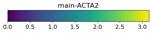
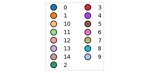
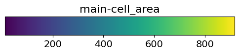
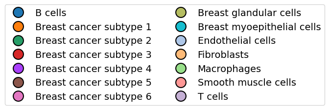
xd.save_colorlegends()

Saving figure to file figures\colorlegend-main-ACTA2.pdf
Saved.
Saving figure to file figures\colorlegend-main-ACTA2.pdf
Saved.
Saving figure to file figures\colorlegend-main-ACTA2.pdf
Saved.
Saving figure to file figures\colorlegend-main-ACTA2.pdf
Saved.