Addition of data segmented with proseg#
Proseg is a transcript-based methodology for probabilistic cell segmentation which can be used to improve the cell segmentation and reduce mixed phenotypes caused by erroneous segmentation of neighboring cells.
## The following code ensures that all functions and init files are reloaded before executions.
%load_ext autoreload
%autoreload 2
from pathlib import Path
from insitupy import InSituData, CACHE
Load data#
insitupy_project = Path(CACHE / "out/demo_insitupy_project")
xd = InSituData.read(insitupy_project)
xd.load_all()
xd
InSituData
Method:		Xenium
Slide ID:	0001879
Sample ID:	Replicate 1
Path:		C:\Users\ge37voy\.cache\InSituPy\out\demo_insitupy_project
Metadata file:	.ispy
    ➤ images
       nuclei:	(25778, 35416)
       CD20:	(25778, 35416)
       HER2:	(25778, 35416)
       HE:	(25778, 35416, 3)
    ➤ cells
       MultiCellData with main layer 'main'
           matrix
               AnnData object with n_obs × n_vars = 156447 × 297
               obs: 'transcript_counts', 'control_probe_counts', 'control_codeword_counts', 'total_counts', 'cell_area', 'nucleus_area', 'n_genes_by_counts', 'n_genes', 'leiden', 'cell_type_dc', 'cell_type_dc_sub', 'cell_type_tacco', 'cell_type_publ'
               var: 'gene_ids', 'feature_types', 'genome', 'n_cells_by_counts', 'mean_counts', 'pct_dropout_by_counts', 'total_counts', 'n_cells'
               uns: 'cell_type_dc_colors', 'cell_type_dc_sub', 'cell_type_dc_sub_colors', 'cell_type_publ_colors', 'cell_type_tacco_colors', 'counts_location', 'leiden', 'leiden_colors', 'log1p', 'neighbors', 'pca', 'umap'
               obsm: 'OT', 'X_pca', 'X_umap', 'annotations', 'ora_estimate', 'ora_pvals', 'regions', 'spatial'
               varm: 'OT', 'PCs'
               layers: 'counts', 'norm_counts'
               obsp: 'connectivities', 'distances'
           boundaries
               BoundariesData object with 2 entries:
                   cells
                   nuclei
    ➤ transcripts
       DataFrame with shape <dask_expr.expr.Scalar: expr=ReadParquetFSSpec(35e32b5).size() // 8, dtype=int64> x 8
    ➤ annotations
       TestKey:	9 annotations, 2 classes ('TestClass','points') ✔
       demo:	4 annotations, 1 class ('None') ✔
       demo2:	5 annotations, 1 class ('None') ✔
       demo3:	7 annotations, 1 class ('None') ✔
       Demo:	28 annotations, 2 classes ('Tumor cells','Stroma') ✔
    ➤ regions
       demo_regions:	3 regions, 3 classes ('Region1','Region2','Region3') ✔
       TMA:	6 regions, 6 classes ('B-2','A-3','B-1','B-3','A-1','A-2') ✔
       Demo:	3 regions, 3 classes ('Region 1','Region 3','Region 2') ✔
Select small region for demonstration#
xdcrop = xd.crop(xlim=(2700,3000), ylim=(2700,3000))
Export transcripts for proseg#
transcripts_out_path = Path(CACHE / "out/transcripts_for_proseg.csv")
transcripts_out_path.parent.mkdir(exist_ok=True)
# export transcripts as csv
xdcrop.transcripts.to_csv(transcripts_out_path, single_file=True)
['C:\\Users\\ge37voy\\.cache\\InSituPy\\out\\transcripts_for_proseg.csv']
Install proseg#
For installation checkout the installation instructions in the proseg Github repository. In brief, proseg is a Rust package and can be installed using:
cargo install proseg
Run proseg#
output_path = transcripts_out_path.parent / "proseg_results"
output_path.mkdir(exist_ok=True)
import subprocess

# Start the process
process = subprocess.Popen([
    'proseg',
    '--xenium', str(transcripts_out_path),
    '--output-path', str(output_path),
    '--min-qv', str(20),
    '--excluded-genes', "^(Deprecated|NegControl|Unassigned|Intergenic|BLANK|antisense)"
    ], stdout=subprocess.PIPE)

# Continuously read the output
while True:
    output = process.stdout.readline()
    if output == b'' and process.poll() is not None:
        break
    if output:
        print(output.decode('utf-8', errors='replace').strip())
Using 16 threads
Read 109974 transcripts
587 cells
310 genes
Estimated full area: 94627.77
Full volume: 557341.2
Using grid size 123.81886. Chunks: 9
Alternative approach: running Proseg in the terminal#
If the previous cell did not execute successfully (e.g., due to spaces in your file path), you can run Proseg directly from the terminal.
Before proceeding, ensure that you have the correct paths to the transcript.csv and for the output_path, then replace the placeholders in the command below:
proseg --xenium /path/to/transcripts.csv --output-path /path/to/output_path
After successfully running the command in the command line, please continue with this tutorial.
Add proseg results to InSituData#
xdcrop.cells.add_proseg(path=output_path)
xdcrop.cells.add_proseg(path=output_path, key="test") # add the data a second time with another key
Convert counts to float32.
Convert counts to float32.
cropped_out = CACHE / "out/cropped"
xdcrop.saveas(cropped_out, overwrite=True)
Reload and visualize data#
xdr = InSituData.read(cropped_out)
xdr.load_all()
# visualize data
xdr.show()
Accessing the proseg data#
Visualization#
In the napari viewer the proseg data can be accessed by selecting the corresponding key from the “Select data” widget:
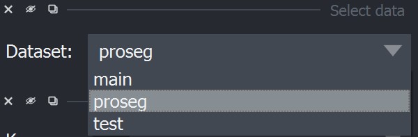
Afterwards the other widgets can be used as usual and access the transcriptomic data stored in .cells[key].matrix.
Working with data layers#
By default the first data layer that is read with functions such as read_xenium is called "main" and is the used as the main_key. The current main key can be accessed with .cells.main_key. When using the syntax .cells.matrix, insitupy automatically selects the main key under .cells[main_key].matrix.
xdr.cells
MultiCellData with main layer 'main'
    matrix
        AnnData object with n_obs × n_vars = 555 × 297
        obs: 'transcript_counts', 'control_probe_counts', 'control_codeword_counts', 'total_counts', 'cell_area', 'nucleus_area', 'n_genes_by_counts', 'n_genes', 'leiden', 'cell_type_dc', 'cell_type_dc_sub', 'cell_type_tacco', 'cell_type_publ'
        var: 'gene_ids', 'feature_types', 'genome', 'n_cells_by_counts', 'mean_counts', 'pct_dropout_by_counts', 'total_counts', 'n_cells'
        uns: 'cell_type_dc_colors', 'cell_type_dc_sub', 'cell_type_dc_sub_colors', 'cell_type_publ_colors', 'cell_type_tacco_colors', 'counts_location', 'leiden', 'leiden_colors', 'log1p', 'neighbors', 'pca', 'umap'
        obsm: 'OT', 'X_pca', 'X_umap', 'annotations', 'ora_estimate', 'ora_pvals', 'regions', 'spatial'
        varm: 'OT', 'PCs'
        layers: 'counts', 'norm_counts'
        obsp: 'connectivities', 'distances'
    boundaries
        BoundariesData object with 2 entries:
            cells
            nuclei

Additional layers with keys: 'proseg', 'test'
xdr.cells.main_key
'main'
xdr.cells.matrix
AnnData object with n_obs × n_vars = 555 × 297
    obs: 'transcript_counts', 'control_probe_counts', 'control_codeword_counts', 'total_counts', 'cell_area', 'nucleus_area', 'n_genes_by_counts', 'n_genes', 'leiden', 'cell_type_dc', 'cell_type_dc_sub', 'cell_type_tacco', 'cell_type_publ'
    var: 'gene_ids', 'feature_types', 'genome', 'n_cells_by_counts', 'mean_counts', 'pct_dropout_by_counts', 'total_counts', 'n_cells'
    uns: 'cell_type_dc_colors', 'cell_type_dc_sub', 'cell_type_dc_sub_colors', 'cell_type_publ_colors', 'cell_type_tacco_colors', 'counts_location', 'leiden', 'leiden_colors', 'log1p', 'neighbors', 'pca', 'umap'
    obsm: 'OT', 'X_pca', 'X_umap', 'annotations', 'ora_estimate', 'ora_pvals', 'regions', 'spatial'
    varm: 'OT', 'PCs'
    layers: 'counts', 'norm_counts'
    obsp: 'connectivities', 'distances'
If you want to access the other layers, you can use the syntax .cells[key]:
xdr.cells["proseg"].matrix
AnnData object with n_obs × n_vars = 587 × 310
    obs: 'centroid_x', 'centroid_y', 'centroid_z', 'fov', 'cluster', 'volume', 'scale', 'population'
    obsm: 'spatial'
xdr.cells["proseg"].boundaries
BoundariesData object with 2 entries:
    cells
Setting different default layer#
If you decide during analysis to use mostly one of the alternative layers for analysis, it can be beneficial to set one of those as default. This can be done using the set_main function:
xdr.cells.set_main("proseg")
xdr.cells
MultiCellData with main layer 'proseg'
    matrix
        AnnData object with n_obs × n_vars = 587 × 310
        obs: 'centroid_x', 'centroid_y', 'centroid_z', 'fov', 'cluster', 'volume', 'scale', 'population'
        obsm: 'spatial'
    boundaries
        BoundariesData object with 2 entries:
            cells

Additional layers with keys: 'main', 'test'