Working with histological annotations and regions#
## The following code ensures that all functions and init files are reloaded before executions.
%load_ext autoreload
%autoreload 2
from pathlib import Path
from insitupy import InSituData, CACHE
Load Xenium data into InSituData object#
Now the Xenium data can be parsed by providing the data path to the InSituPy project folder
insitupy_project = Path(CACHE / "out/demo_insitupy_project")
xd = InSituData.read(insitupy_project)
xd
InSituData
Method:		Xenium
Slide ID:	0001879
Sample ID:	Replicate 1
Path:		C:\Users\ge37voy\.cache\InSituPy\out\demo_insitupy_project
Metadata file:	.ispy

No modalities loaded.
Here we only load the images and cells modalities. Since InSitupy v0.6.2 transcripts are loaded lazily, so it would be also just as fast to use load_all() here.
xd.load_images()
xd.load_cells()
xd
InSituData
Method:		Xenium
Slide ID:	0001879
Sample ID:	Replicate 1
Path:		C:\Users\ge37voy\.cache\InSituPy\out\demo_insitupy_project
Metadata file:	.ispy
    ➤ images
       nuclei:	(25778, 35416)
       CD20:	(25778, 35416)
       HER2:	(25778, 35416)
       HE:	(25778, 35416, 3)
    ➤ cells
       MultiCellData with main layer 'main'
           matrix
               AnnData object with n_obs × n_vars = 157600 × 297
               obs: 'transcript_counts', 'control_probe_counts', 'control_codeword_counts', 'total_counts', 'cell_area', 'nucleus_area', 'n_genes_by_counts', 'n_genes', 'leiden'
               var: 'gene_ids', 'feature_types', 'genome', 'n_cells_by_counts', 'mean_counts', 'pct_dropout_by_counts', 'total_counts', 'n_cells'
               uns: 'leiden', 'leiden_colors', 'log1p', 'neighbors', 'pca', 'umap'
               obsm: 'X_pca', 'X_umap', 'spatial'
               varm: 'PCs'
               layers: 'counts', 'norm_counts'
               obsp: 'connectivities', 'distances'
           boundaries
               BoundariesData object with 2 entries:
                   cells
                   nuclei
Create Annotations#
For the analysis of spatial transcriptomic datasets, the inclusion of annotations from experts in disease pathology is key. Here, we demonstrate two ways to annotate Xenium data:
Within
InSituPyusing thenapariviewer.Using QuPath.
Key Concepts#
Annotations in InSituPy#
Annotations consist of polygons, points or lines.
Each polygon is assigned to a certain class (e.g., “tumor cells”, “immune cells”, “stroma”, etc.).
Each polygon is also assigned a key (e.g., the name of the pathologist doing the annotations).
Classes within one key do not have to be unique (multiple annotations could contain tumor cells).
A unique identifier is used to differentiate between the polygons.
Regions in InSituPy#
Regions also consist of polygons.
Regions have a key for a cohesive group of polygons (e.g. “TMA”).
Each polygon within one key is required to have a unique name (e.g. “TMA A-1”).
Regions can delineate:
The positions of TMA cores.
The positions of different tissue sections.
Regions of interest within the same dataset.
1. In napari viewer#
First visualize the Xenium data using .show().
xd.show()
A new annotation layer can be added using the “Add geometries” widget on the bottom right.
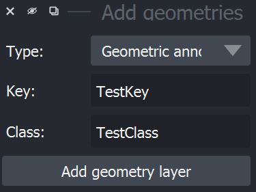
As described above, InSituPy differentiates between “regions” and histological “annotations”. Since napari creates separate layers for point and shape annotations, the “annotations” are split further into two subtypes, resulting in a total of three possible geometry types one can chose from:
Geometric annotations

Point annotations

Region

Since InSituPy uses different icons to differentiate between the types, it is important to add the geometries via this widget and not via the normal napari annotation panel.
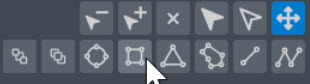
After adding the respective shapes layer, one can now add shapes using the tool box of napari on the top left. E.g. for a geometric annotation, the tool set would look like this:
After adding the geometries, they can be imported into the InSituPy object using .store_geometries():
xd.store_geometries()
Added 5 new annotations to key 'TestKey'
Added 4 new annotations to existing key 'TestKey'
xd
InSituData
Method:		Xenium
Slide ID:	0001879
Sample ID:	Replicate 1
Path:		C:\Users\ge37voy\.cache\InSituPy\out\demo_insitupy_project
Metadata file:	.ispy
    ➤ images
       nuclei:	(25778, 35416)
       CD20:	(25778, 35416)
       HER2:	(25778, 35416)
       HE:	(25778, 35416, 3)
    ➤ cells
       MultiCellData with main layer 'main'
           matrix
               AnnData object with n_obs × n_vars = 157600 × 297
               obs: 'transcript_counts', 'control_probe_counts', 'control_codeword_counts', 'total_counts', 'cell_area', 'nucleus_area', 'n_genes_by_counts', 'n_genes', 'leiden'
               var: 'gene_ids', 'feature_types', 'genome', 'n_cells_by_counts', 'mean_counts', 'pct_dropout_by_counts', 'total_counts', 'n_cells'
               uns: 'leiden', 'leiden_colors', 'log1p', 'neighbors', 'pca', 'umap'
               obsm: 'X_pca', 'X_umap', 'spatial'
               varm: 'PCs'
               layers: 'counts', 'norm_counts'
               obsp: 'connectivities', 'distances'
           boundaries
               BoundariesData object with 2 entries:
                   cells
                   nuclei
    ➤ annotations
       TestKey:	9 annotations, 2 classes ('TestClass','points')
xd.annotations["TestKey"].head()
| objectType | geometry | name | color | origin | layer_type | |
|---|---|---|---|---|---|---|
| id | ||||||
| d400e615-5fe0-4793-8622-60f8de3e7840 | annotation | POLYGON ((2428.52808 1676.14758, 2300.68945 19... | TestClass | [255, 0, 0] | manual | Shapes |
| ac177acf-a5a9-4e17-8a73-74cf58560281 | annotation | POLYGON ((3802.79321 1963.78455, 3515.15649 23... | TestClass | [255, 0, 0] | manual | Shapes |
| 426990f2-dfa8-4bec-ac35-aa641c448f30 | annotation | POLYGON ((4761.58301 2027.70386, 5816.25195 20... | TestClass | [255, 0, 0] | manual | Shapes |
| c0f40469-40f4-4102-a1c0-3aabc3608c0b | annotation | LINESTRING (1373.85938 2139.56274, 1837.27441 ... | TestClass | [255, 0, 0] | manual | Shapes |
| 4b232f1a-0b05-438d-87f5-1fc6958373f9 | annotation | LINESTRING (1054.26282 2650.91724, 2332.64917 ... | TestClass | [255, 0, 0] | manual | Shapes |
Export annotations or regions#
To export annotations or regions, one can save the AnnotationsData or RegionsData object as .geojson file.
xd.annotations.save(path=CACHE / "out/annotations_export", overwrite=True)
2. Create annotations in QuPath#
To create annotations in QuPath, follow these steps:
Export the registered HE image as OME-TIFF by setting
as_zarr=False:
xd.images.save(CACHE / "out/image_export", keys_to_save="HE", as_zarr=False, overwrite=True)
Open the exported image in QuPath and start with the annotations. Documentations on QuPath can be found here.
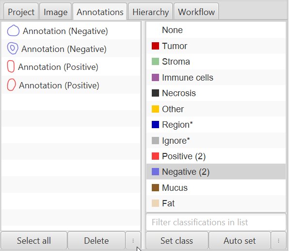
Select an annotation tool from the bar on the top left:

Add as many annotations as you want and label them by setting classes in the annotation list. Do not forget to press the “Set class” button:
Export annotations using
File > Export objects as GeoJSON. TickPretty JSONto get an easily readable JSON file. The file name needs to have following structure:annotation-{slide_id}__{sample_id}__{annotation_label}.
Import annotations into InSituData#
For demonstration purposes, we created dummy annotation files in ./demo_annotations/. To add the annotations to InSituData follow the steps below.
3. Create regions in QuPath#
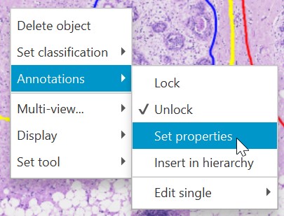
For creating regions, one can use the same annotation tools as described above. But instead of setting a class for the annotation, you can name the region by double-clicking on it, and selecting “Set Properties”:
For export, regions can then be selected and exported in the same way as described above for annotations.
Import annotations and regions#
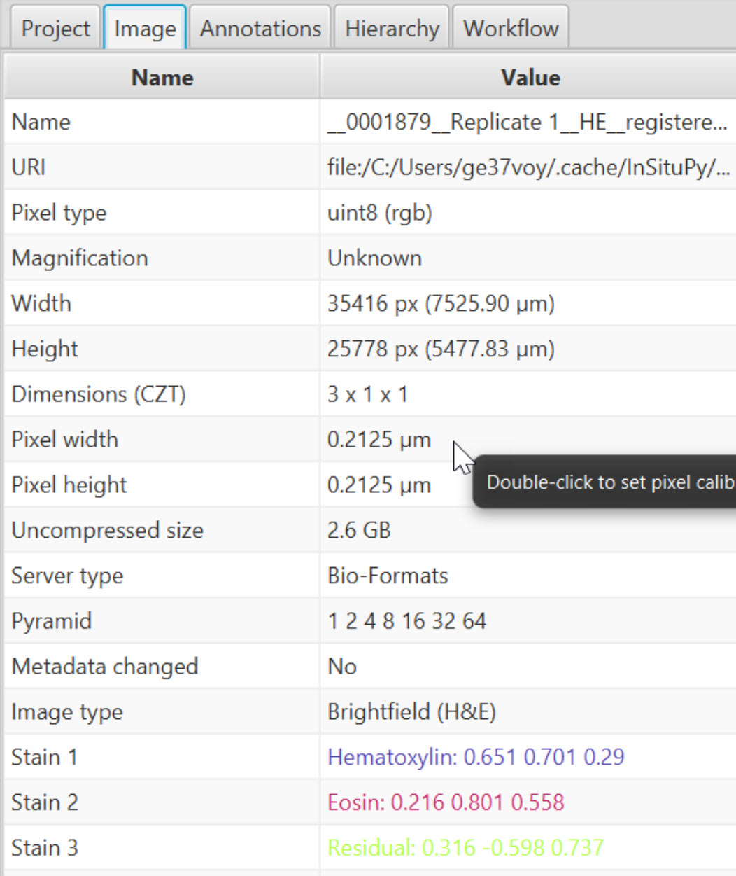
Since annotations could have been done on images with different resolutions, it is important to specify the pixel_size during the import. In standard Xenium experiments the pixel size is 0.2125 µm but if the images were downscaled before the annotation, this value might differ.
In QuPath the pixel size and other image metadata can be looked up under “Image” and “Pixel width” or “Pixel height”:
xd.import_annotations(
    files=[
        "../../demo_data/demo_annotations/annotations-0001879__Replicate 1__demo.geojson",
        "../../demo_data/demo_annotations/annotations-0001879__Replicate 1__demo2.geojson",
        "../../demo_data/demo_annotations/annotations-mixed_types.geojson"
           ],
    keys=["demo", "demo2", "demo3"],
    scale_factor=0.2125
    )
xd.annotations["demo"]
| objectType | classification | geometry | origin | name | layer_type | |
|---|---|---|---|---|---|---|
| id | ||||||
| bd3aacca-1716-4df8-91dd-bf8f6413a7bd | annotation | { "name": "Positive", "color": [ 250, 62, 62 ] } | POLYGON ((1883.3875 2297.975, 1883.3875 2300.1... | file | None | Shapes |
| 69814505-4059-42cd-8df2-752f7eb0810d | annotation | { "name": "Positive", "color": [ 250, 62, 62 ] } | POLYGON ((2782.9 2654.55, 2777.885 2655.0175, ... | file | None | Shapes |
| 1957cd32-0a21-4b45-9dae-ecf236217140 | annotation | { "name": "Negative", "color": [ 112, 112, 225... | POLYGON ((6582.24275 4874.325, 6583.675 4874.3... | file | None | Shapes |
| 19d2197a-1b8e-456f-8223-fba74641ac1c | annotation | { "name": "Negative", "color": [ 112, 112, 225... | POLYGON ((6622.5625 3486.7, 6619.1625 3487.125... | file | None | Shapes |
xd.annotations["demo2"]
| objectType | classification | geometry | origin | name | layer_type | |
|---|---|---|---|---|---|---|
| id | ||||||
| 1970eccb-ad38-4b4b-b7a8-54509027b57d | annotation | { "name": "Negative", "color": [ 112, 112, 225... | POLYGON ((5380.2875 827.05, 5379.0125 827.475,... | file | None | Shapes |
| a3b32cce-1bb9-4a6f-b1d1-9e0c44420cfa | annotation | { "name": "Positive", "color": [ 250, 62, 62 ] } | POLYGON ((6576.875 2306.6875, 6575.6 2307.1125... | file | None | Shapes |
| 92bfe928-a21f-4864-b7cb-f0d300113d88 | annotation | { "name": "Other", "color": [ 255, 200, 0 ] } | MULTIPOLYGON (((4575.975 4152.4625, 4575.975 4... | file | None | Shapes |
| a6c17a54-6839-40b2-8531-c9227635f344 | annotation | { "name": "Other", "color": [ 255, 200, 0 ] } | POLYGON ((1381.4625 3639.275, 1380.1875 3639.7... | file | None | Shapes |
| e78efe2f-d185-4ab6-9cc9-6621897f3662 | annotation | { "name": "Negative", "color": [ 112, 112, 225... | POLYGON ((6272.92138 3936.1375, 6263.65 3945.2... | file | None | Shapes |
xd.annotations["demo3"]
| objectType | classification | geometry | origin | name | layer_type | |
|---|---|---|---|---|---|---|
| id | ||||||
| 8f57c3c3-2216-48b7-99bd-aba12d8c3c41 | annotation | { "name": "Stroma", "color": [ 150, 200, 150 ] } | POLYGON ((3828.4 2261.74375, 3827.8135 2274.22... | file | None | Shapes |
| 7e8f8db4-81d4-472e-8e93-0fc756df87aa | annotation | { "name": "Stroma", "color": [ 150, 200, 150 ] } | POLYGON ((2618.425 1436.075, 2618.07225 1436.1... | file | None | Shapes |
| 38a48ddb-f33c-4c61-b996-330b25d84081 | annotation | { "name": "Necrosis", "color": [ 50, 50, 50 ] } | LINESTRING (3600.5575 1648.7535, 3878.03575 13... | file | None | Shapes |
| eee244c9-e919-41ae-bb91-44c7abcc0cec | annotation | { "name": "Immune cells", "color": [ 160, 90, ... | LINESTRING (2483.6235 1334.39588, 2855.93412 1... | file | None | Shapes |
| e3d4c0b6-0998-4692-ab7d-f580f713e275 | annotation | None | POINT (5096.23663 1632.56312) | file | None | Points |
| e9105240-3b35-489e-994f-e8f9c4786516 | annotation | { "name": "Stroma", "color": [ 150, 200, 150 ] } | MULTIPOINT (4219.655 1650.71912, 4261.94675 13... | file | None | Points |
| 2802df97-78ad-44ac-8e6b-d9b9406c8e3f | annotation | { "name": "Tumor", "color": [ 200, 0, 0 ] } | MULTIPOINT (3372.7915 2005.41562, 3530.0415 20... | file | None | Points |
Load regions#
Regions can be created in QuPath either as described above or using tools like the TMA dearrayer. They are also exported as objects as annotations but different to annotations they do not have a classification and each name of a region has to be unique.
In the following demo regions are read. One of the region files has non-unique names to demonstrate the warning that appears in this case.
In regions classes have to be unique#
When reading an “Annotation” .geojson as shown below, the import_regions function throws an error indicating that in regions only one geometry per class is allowed. Further, only normal polygons (shapely.Polygon-typed) are allowed. Any other types of geometries (Points, Lines, MultiPolygons, …) are skipped.
xd.import_regions(
    files=[
        "../../demo_data/demo_annotations/annotations-mixed_types.geojson"
        ],
    keys=['test'],
    scale_factor=0.2125
    )
Multiple regions can be imported simultaneously.
xd.import_regions(
    files=[
        "../../demo_data/demo_regions/regions-0001879__Replicate 1__demo_regions.geojson",
        "../../demo_data/demo_regions/regions-0001879__Replicate 1__TMA.geojson",
        ],
    keys=['demo_regions', 'TMA'],
    scale_factor=0.2125
    )
Properties of the anotations and regions modalities can be inspected in the InSituData representation:
xd
InSituData
Method:		Xenium
Slide ID:	0001879
Sample ID:	Replicate 1
Path:		C:\Users\ge37voy\.cache\InSituPy\out\demo_insitupy_project
Metadata file:	.ispy
    ➤ images
       nuclei:	(25778, 35416)
       CD20:	(25778, 35416)
       HER2:	(25778, 35416)
       HE:	(25778, 35416, 3)
    ➤ cells
       MultiCellData with main layer 'main'
           matrix
               AnnData object with n_obs × n_vars = 157600 × 297
               obs: 'transcript_counts', 'control_probe_counts', 'control_codeword_counts', 'total_counts', 'cell_area', 'nucleus_area', 'n_genes_by_counts', 'n_genes', 'leiden'
               var: 'gene_ids', 'feature_types', 'genome', 'n_cells_by_counts', 'mean_counts', 'pct_dropout_by_counts', 'total_counts', 'n_cells'
               uns: 'leiden', 'leiden_colors', 'log1p', 'neighbors', 'pca', 'umap'
               obsm: 'X_pca', 'X_umap', 'spatial'
               varm: 'PCs'
               layers: 'counts', 'norm_counts'
               obsp: 'connectivities', 'distances'
           boundaries
               BoundariesData object with 2 entries:
                   cells
                   nuclei
    ➤ annotations
       TestKey:	9 annotations, 2 classes ('TestClass','points')
       demo:	4 annotations, 1 class ('None')
       demo2:	5 annotations, 1 class ('None')
       demo3:	7 annotations, 1 class ('None')
    ➤ regions
       demo_regions:	3 regions, 3 classes ('Region1','Region2','Region3')
       TMA:	6 regions, 6 classes ('B-2','A-3','B-1','B-3','A-1','A-2')
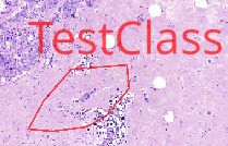
Visualization of annotations and regions using napari viewer#
Ìf the InSituData object only contains .annotations or .regions attributes, one can choose between the “Add geometries” and “Show geometries” widgets:

Annotations and regions stored in the InSituData object can be visualized using the “Show geometries” widget:
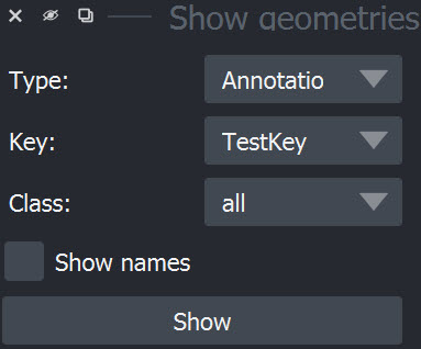
To show the names of the annotations, tick “Show names”:
xd.show()
Assign annotations to observations#
To use the annotations in analyses (e.g. to select only observations within a certain annotation or compare gene expression between different annotations) one can use the assign_annotations function. It adds columns containing the annotation class to xd.matrix.obs. The column has the syntax annotation-{Label} and if an observation is not part of any annotation within this label, it contains NaN.
xd.assign_annotations(overwrite=True)
Using CellData from MultiCellData layer 'main'.
Assigning key 'TestKey'...
Added results to `.cells['main'].matrix.obsm['annotations']
Assigning key 'demo'...
Added results to `.cells['main'].matrix.obsm['annotations']
Assigning key 'demo2'...
Added results to `.cells['main'].matrix.obsm['annotations']
Assigning key 'demo3'...
Added results to `.cells['main'].matrix.obsm['annotations']
xd.assign_regions()
Using CellData from MultiCellData layer 'main'.
Assigning key 'demo_regions'...
Added results to `.cells['main'].matrix.obsm['regions']
Assigning key 'TMA'...
Added results to `.cells['main'].matrix.obsm['regions']
xd
InSituData
Method:		Xenium
Slide ID:	0001879
Sample ID:	Replicate 1
Path:		C:\Users\ge37voy\.cache\InSituPy\out\demo_insitupy_project
Metadata file:	.ispy
    ➤ images
       nuclei:	(25778, 35416)
       CD20:	(25778, 35416)
       HER2:	(25778, 35416)
       HE:	(25778, 35416, 3)
    ➤ cells
       MultiCellData with main layer 'main'
           matrix
               AnnData object with n_obs × n_vars = 157600 × 297
               obs: 'transcript_counts', 'control_probe_counts', 'control_codeword_counts', 'total_counts', 'cell_area', 'nucleus_area', 'n_genes_by_counts', 'n_genes', 'leiden'
               var: 'gene_ids', 'feature_types', 'genome', 'n_cells_by_counts', 'mean_counts', 'pct_dropout_by_counts', 'total_counts', 'n_cells'
               uns: 'leiden', 'leiden_colors', 'log1p', 'neighbors', 'pca', 'umap'
               obsm: 'X_pca', 'X_umap', 'spatial', 'annotations', 'regions'
               varm: 'PCs'
               layers: 'counts', 'norm_counts'
               obsp: 'connectivities', 'distances'
           boundaries
               BoundariesData object with 2 entries:
                   cells
                   nuclei
    ➤ annotations
       TestKey:	9 annotations, 2 classes ('TestClass','points') ✔
       demo:	4 annotations, 1 class ('None') ✔
       demo2:	5 annotations, 1 class ('None') ✔
       demo3:	7 annotations, 1 class ('None') ✔
    ➤ regions
       demo_regions:	3 regions, 3 classes ('Region1','Region2','Region3') ✔
       TMA:	6 regions, 6 classes ('B-2','A-3','B-1','B-3','A-1','A-2') ✔
After assigning the annotations, the already analyzed labels analyzed are marked with a ✔:
xd.regions["demo_regions"]
| objectType | name | geometry | origin | layer_type | |
|---|---|---|---|---|---|
| id | |||||
| 2d0da635-c408-459f-9178-839097fe5a98 | annotation | Region1 | POLYGON ((1564.425 1321.9625, 2267.8 1321.9625... | file | Shapes |
| ce6c2342-620d-4f44-be03-68a4454e9b33 | annotation | Region2 | POLYGON ((4541.7625 1356.3875, 5613.825 1356.3... | file | Shapes |
| 70a125ec-c53e-469b-8927-efe224e504c1 | annotation | Region3 | POLYGON ((2110.7625 2708.3125, 3387.675 2708.3... | file | Shapes |
Following cells show examples how to explore the assigned annotations:
xd.cells.matrix.obsm['annotations']['demo2']
2         unassigned
5         unassigned
8         unassigned
10        unassigned
13        unassigned
             ...
167776    unassigned
167777    unassigned
167778    unassigned
167779    unassigned
167780    unassigned
Name: demo2, Length: 157600, dtype: object
# print number of cells within each annotation
annots = xd.cells.matrix.obsm['annotations']['demo2']
annots.value_counts()
demo2
unassigned    148458
None            9142
Name: count, dtype: int64
# show geopandas dataframe for one annotation
xd.annotations["demo2"]
| objectType | classification | geometry | origin | name | layer_type | |
|---|---|---|---|---|---|---|
| id | ||||||
| 1970eccb-ad38-4b4b-b7a8-54509027b57d | annotation | { "name": "Negative", "color": [ 112, 112, 225... | POLYGON ((5380.2875 827.05, 5379.0125 827.475,... | file | None | Shapes |
| a3b32cce-1bb9-4a6f-b1d1-9e0c44420cfa | annotation | { "name": "Positive", "color": [ 250, 62, 62 ] } | POLYGON ((6576.875 2306.6875, 6575.6 2307.1125... | file | None | Shapes |
| 92bfe928-a21f-4864-b7cb-f0d300113d88 | annotation | { "name": "Other", "color": [ 255, 200, 0 ] } | MULTIPOLYGON (((4575.975 4152.4625, 4575.975 4... | file | None | Shapes |
| a6c17a54-6839-40b2-8531-c9227635f344 | annotation | { "name": "Other", "color": [ 255, 200, 0 ] } | POLYGON ((1381.4625 3639.275, 1380.1875 3639.7... | file | None | Shapes |
| e78efe2f-d185-4ab6-9cc9-6621897f3662 | annotation | { "name": "Negative", "color": [ 112, 112, 225... | POLYGON ((6272.92138 3936.1375, 6263.65 3945.2... | file | None | Shapes |
Save imported annotations in InSituPy project#
xd.save()
Updating project in C:\Users\ge37voy\.cache\InSituPy\out\demo_insitupy_project
	Updating cells...
	Updating annotations...
	Updating regions...
Saved.