Spatial plotting functionalities#
This notebook shows the insitupy plotting functionalities. It assumes that the previous steps of the demo notebooks such as preprocessing, import of annotations and regions and cell type annotation have been run.
## The following code ensures that all functions and init files are reloaded before executions.
%load_ext autoreload
%autoreload 2
from pathlib import Path
from insitupy import InSituData, CACHE
import insitupy as isp
Load data#
insitupy_project = Path(CACHE / "out/demo_insitupy_project")
xd = InSituData.read(insitupy_project)
xd.load_all()
xd
InSituData
Method:		Xenium
Slide ID:	0001879
Sample ID:	Replicate 1
Path:		C:\Users\ge37voy\.cache\InSituPy\out\demo_insitupy_project

    ➤ images
       CD20:	(25778, 35416)
       HE:	(25778, 35416, 3)
       HER2:	(25778, 35416)
       nuclei:	(25778, 35416)
    ➤ cells
       MultiCellData with main layer 'main'
           matrix
               AnnData object with n_obs × n_vars = 156447 × 297
               obs: 'transcript_counts', 'control_probe_counts', 'control_codeword_counts', 'total_counts', 'cell_area', 'nucleus_area', 'n_genes_by_counts', 'n_genes', 'leiden', 'cell_type_dc', 'cell_type_dc_sub', 'cell_type_tacco', 'cell_type_publ_x', 'cell_type_publ_y', 'cell_type_dc_sub_final', 'cell_type_publ'
               var: 'gene_ids', 'feature_types', 'genome', 'n_cells_by_counts', 'mean_counts', 'pct_dropout_by_counts', 'total_counts', 'n_cells'
               uns: 'cell_type_dc_colors', 'cell_type_dc_sub', 'cell_type_dc_sub_colors', 'cell_type_dc_sub_final_colors', 'cell_type_publ_colors', 'cell_type_tacco_colors', 'counts_location', 'leiden', 'leiden_colors', 'log1p', 'neighbors', 'pca', 'umap'
               obsm: 'OT', 'X_pca', 'X_umap', 'annotations', 'ora_estimate', 'ora_pvals', 'regions', 'spatial'
               varm: 'OT', 'PCs'
               layers: 'counts', 'norm_counts'
               obsp: 'connectivities', 'distances'
           boundaries
               BoundariesData object with 2 entries:
                   cells
                   nuclei
    ➤ transcripts
       DataFrame with shape <dask_expr.expr.Scalar: expr=ReadParquetFSSpec(8ccd9b1).size() // 8, dtype=int64> x 8
    ➤ annotations
       TestKey:	5 annotations, 2 classes ('TestClass', 'test') ✔
       demo:	28 annotations, 2 classes ('Stroma', 'Tumor cells') ✔
       demo2:	5 annotations, 3 classes ('Negative', 'Other', 'Positive') ✔
       demo3:	7 annotations, 5 classes ('Immune cells', 'Necrosis', 'Stroma', 'Tumor', 'unclassified') ✔
       Demo:	28 annotations, 2 classes ('Stroma', 'Tumor cells') ✔
       Janesick:	18 annotations, 3 classes ('DCIS #1', 'DCIS #2', 'Invasive')
       Katja:	18 annotations, 4 classes ('DCIS', 'DCIS intermediate', 'DCIS with stromal reaction', 'Invasive') ✔
    ➤ regions
       demo_regions:	3 regions, 3 classes ('Region1', 'Region2', 'Region3') ✔
       TMA:	6 regions, 6 classes ('A-1', 'A-2', 'A-3', 'B-1', 'B-2', 'B-3') ✔
       Demo:	3 regions, 3 classes ('Region 1', 'Region 2', 'Region 3') ✔
       Katja:	4 regions, 4 classes ('Region 1', 'Region 2', 'Region 3', 'Region 4') ✔
Sample-level or experimental level plotting of expression data#
#from insitupy.plotting import spatial
import insitupy as isp
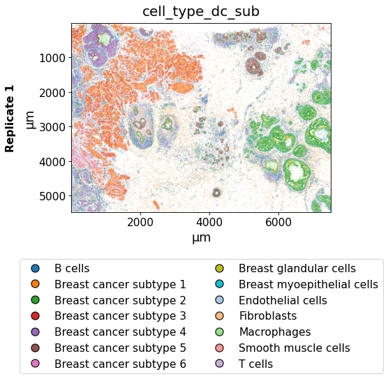
Using the keys argument, one or multiple keys can be selected to be displayed.
isp.pl.spatial(xd, keys="cell_type_dc_sub")
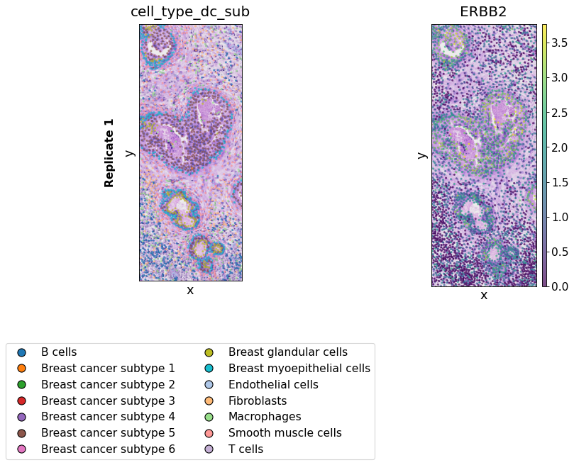
isp.pl.spatial(xd, keys=["cell_type_dc_sub", "ERBB2"])
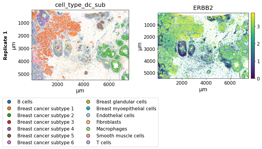
The savepath argument can be used to save the plot in a certain path. The filename extension determines the format of the output image. When saving as .pdf long saving times can occur due to the large number of data points.
isp.pl.spatial(xd,
               keys=["cell_type_dc_sub", "ERBB2"],
               savepath="figures/spatial-demo.png"
               )
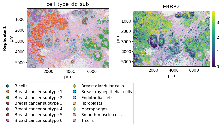
The image_key argument can be used to select a image to be displayed in the background.
isp.pl.spatial(xd, keys=["cell_type_dc_sub", "ERBB2"],
               image_key="HE")
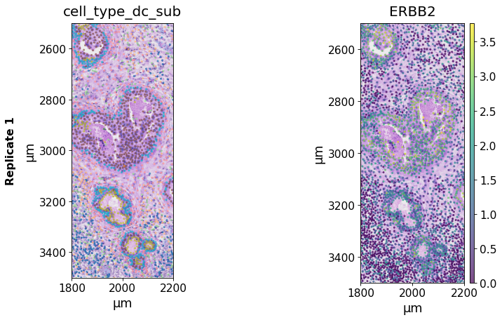
The xlim/ylim parameters can be used to zoom into the images and plot only selected regions and the spot_size argument to adapt the size of the spots. Further, the opacity of the spots can be adapted using alpha.
from insitupy.plotting.spatial import PlotConfig, LayoutConfig, DataConfig

# to further configure the plot one can use the configuration classes: PlotConfig, LayoutConfig and DataConfig
plot_config = PlotConfig(legend_max_per_col=8, show_scale=False)

# all possible configurations can be shown with `show_all()`:
plot_config.show_all()
Configuration parameters for PlotConfig:
	xlim: None
	ylim: None
	spot_size: 10
	alpha: 1.0
	cmap: viridis
	palette: <matplotlib.colors.ListedColormap object at 0x0000016B32947910>
	spot_type: o
	background_color: white
	cmap_center: None
	normalize: None
	show_legend: True
	legend_max_per_col: 8
	clb_title: None
	annotations_mode: outlined
	crange: None
	crange_type: upper_percentile
	origin_zero: False
	label_size: 16
	show_title: True
	title_size: 18
	show_scale: False
	tick_label_size: 14
	pixelwidth_per_subplot: 200
	histogram_setting: auto
# a configurations file can then be used to customize the plot:
isp.pl.spatial(xd, keys=["cell_type_dc_sub", "ERBB2"],
             spot_size=8, alpha=0.7,
             xlim=(1800, 2200), ylim=(2500, 3500),
             image_key="HE",
             plot_config=plot_config
             )
One can also deactivate plotting of the color legend:
plot_config = PlotConfig(show_legend=False)

# a configurations file can then be used to customize the plot:
isp.pl.spatial(xd, keys=["cell_type_dc_sub", "ERBB2"],
             spot_size=8, alpha=0.7,
             xlim=(1800, 2200), ylim=(2500, 3500),
             image_key="HE",
             plot_config=plot_config
             )
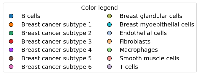
Here is how one can plot the color legend separately:
# extract the color mapping from the anndata object
mapping = dict(zip(xd.cells.matrix.obs['cell_type_dc_sub'].cat.categories,
                   xd.cells.matrix.uns['cell_type_dc_sub_colors']))

# plot color legend
isp.pl.colorlegend(mapping=mapping)
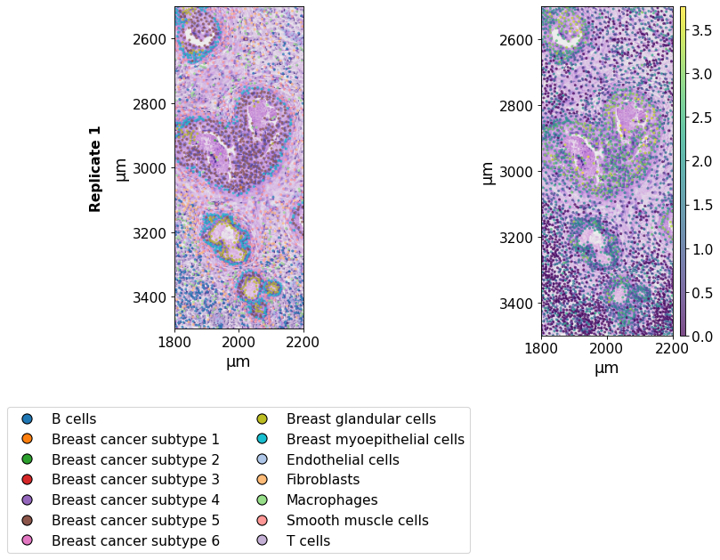
plot_config = PlotConfig(show_title=False)

# a configurations file can then be used to customize the plot:
isp.pl.spatial(xd, keys=["cell_type_dc_sub", "ERBB2"],
             spot_size=8, alpha=0.7,
             xlim=(1800, 2200), ylim=(2500, 3500),
             image_key="HE",
             plot_config=plot_config
             )
When working with an InSituExperiment object for multi-sample analysis, one can directly plot all datasets within the InSituExperiment object. For details on generating InSituExperiment objects and working with them see this notebook.
from insitupy import InSituExperiment
First, we generate an InSituExperiment object.
exp = InSituExperiment.from_regions(
    data=xd, region_key="TMA"
)
A-1
A-2
A-3
B-1
B-2
B-3
And then we can use the spatial function directly on the InSituExperiment object. The name_column argument can be used to determine the column in the .metadata dataframe to be used for naming the plot.
exp.metadata
| uid | slide_id | sample_id | region_key | region_name | |
|---|---|---|---|---|---|
| 0 | 4a8dde28 | 0001879 | Replicate 1 | TMA | A-1 |
| 1 | d7467790 | 0001879 | Replicate 1 | TMA | A-2 |
| 2 | 234b144c | 0001879 | Replicate 1 | TMA | A-3 |
| 3 | 4d9a8920 | 0001879 | Replicate 1 | TMA | B-1 |
| 4 | 4f795374 | 0001879 | Replicate 1 | TMA | B-2 |
| 5 | 5fe17272 | 0001879 | Replicate 1 | TMA | B-3 |
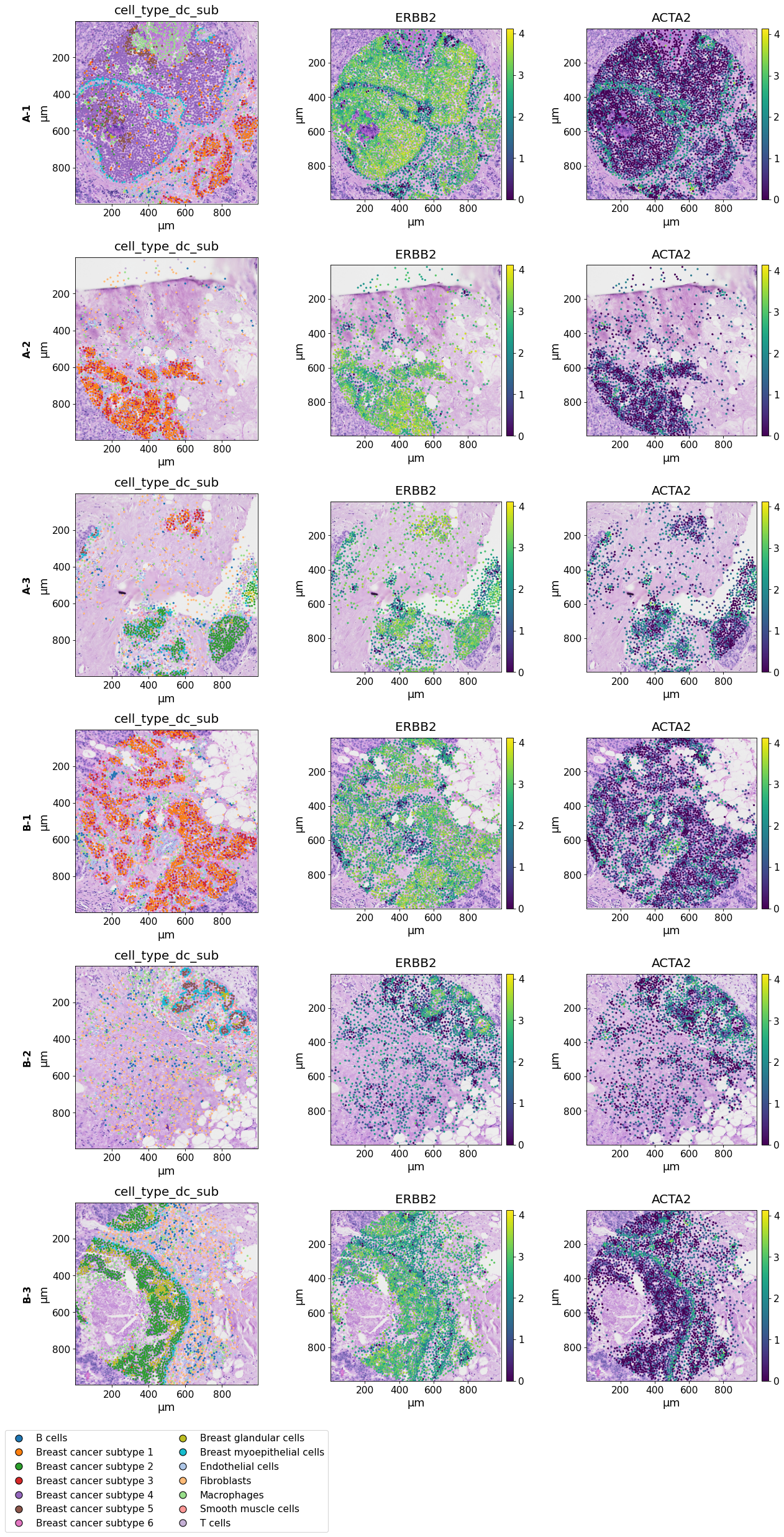
When using both multiple datasets and multiple keys the plots are represented in a grid layout. The wspace and hspace parameters in LayoutConfig can be used to increase the spacing between the subplots in case they are overlapping using the default parameters. Further, the name_column parameter in DataConfig can be used to determine which column in .metadata of the InSituExperiment should be used to infer the title of the different datasets. If using the default None, the title is retrieved from the column "sample_id".
data_config = DataConfig(name_column="region_name")
layout_config = LayoutConfig(wspace=0.4, hspace=0.2)

isp.pl.spatial(exp,
              keys=["cell_type_dc_sub", "ERBB2", "ACTA2"], image_key="HE",
              data_config=data_config,
              layout_config=layout_config,
              savepath="figures/spatial-demo-regions.png"
              )
Key 'cell_type_dc_sub' found already in `exp.colors`. To overwrite it, run `sync_colors` with `overwrite=True`.
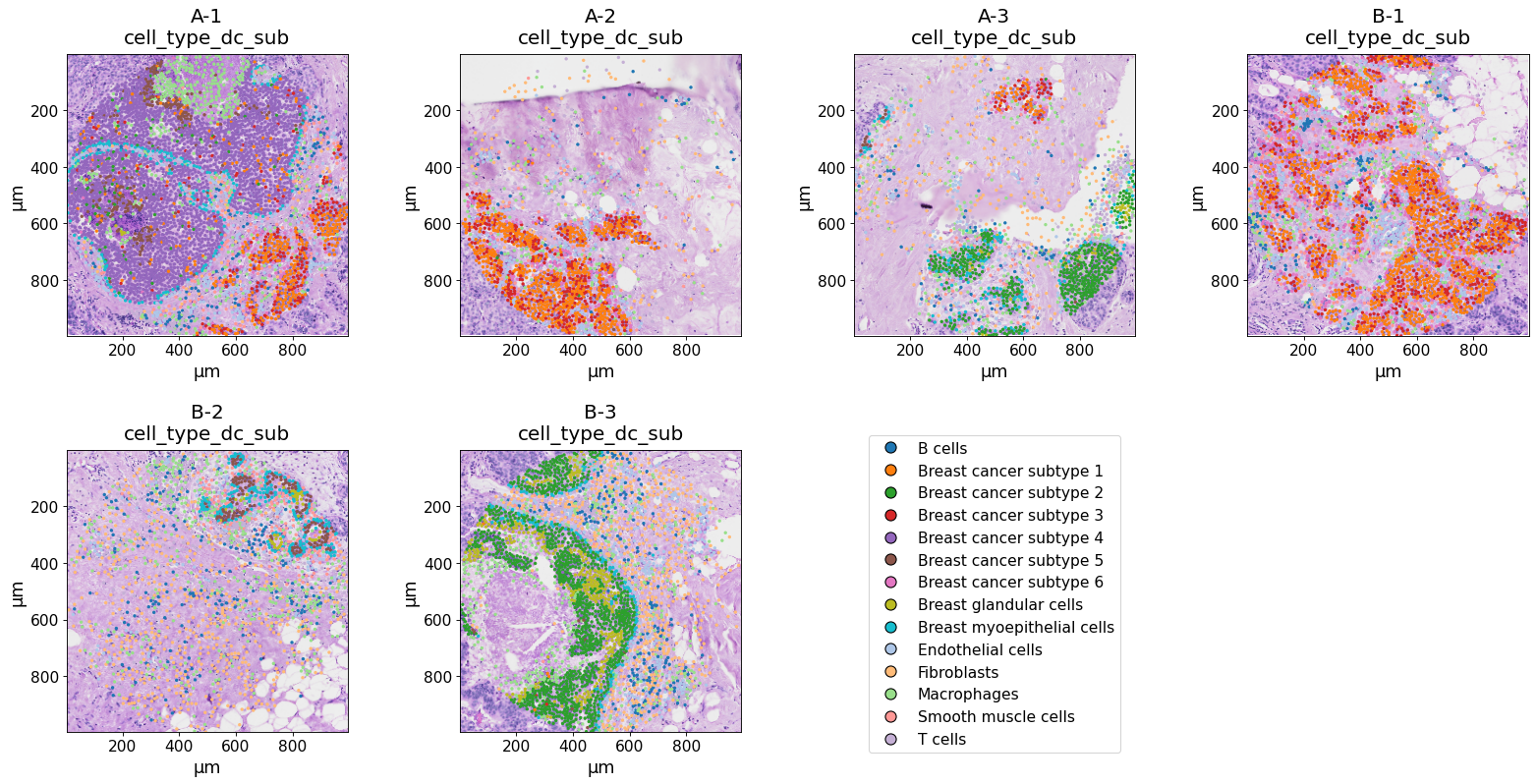
When using only multiple datasets but only one key, they are listed next to each other.
data_config = DataConfig(name_column="region_name")
plot_config = PlotConfig(legend_max_per_col=14)

isp.pl.spatial(exp, keys=["cell_type_dc_sub"],
               image_key="HE",
               data_config=data_config,
               plot_config=plot_config
               )
Key 'cell_type_dc_sub' found already in `exp.colors`. To overwrite it, run `sync_colors` with `overwrite=True`.
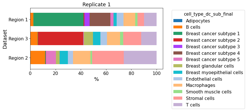
Cellular composition plotting#
from insitupy.plotting import cellular_composition
cellular_composition(
    data=xd, cell_type_col="cell_type_dc_sub_final",
    geom_key="Demo", modality="regions", max_cols=1,
    #savepath="figures/cell_composition_regions_Demo_publ.pdf"
)
Since only one dataset is given, all regions are plotted into one figure.
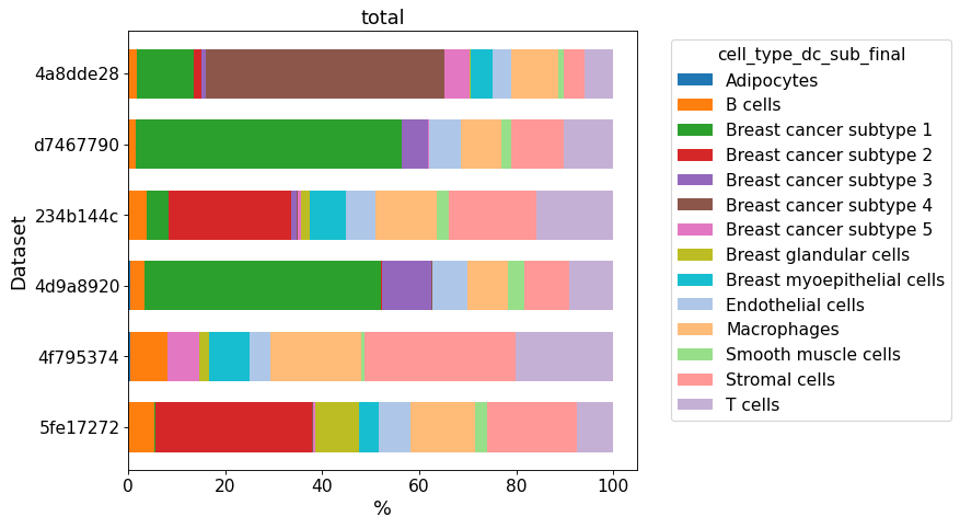
When plotting an InSituExperiment object, the datasets are compared against each other.
cellular_composition(
    data=exp, cell_type_col="cell_type_dc_sub_final",
)
Synchronized colors for key 'cell_type_dc_sub_final' and palette 'tab20_mod'.
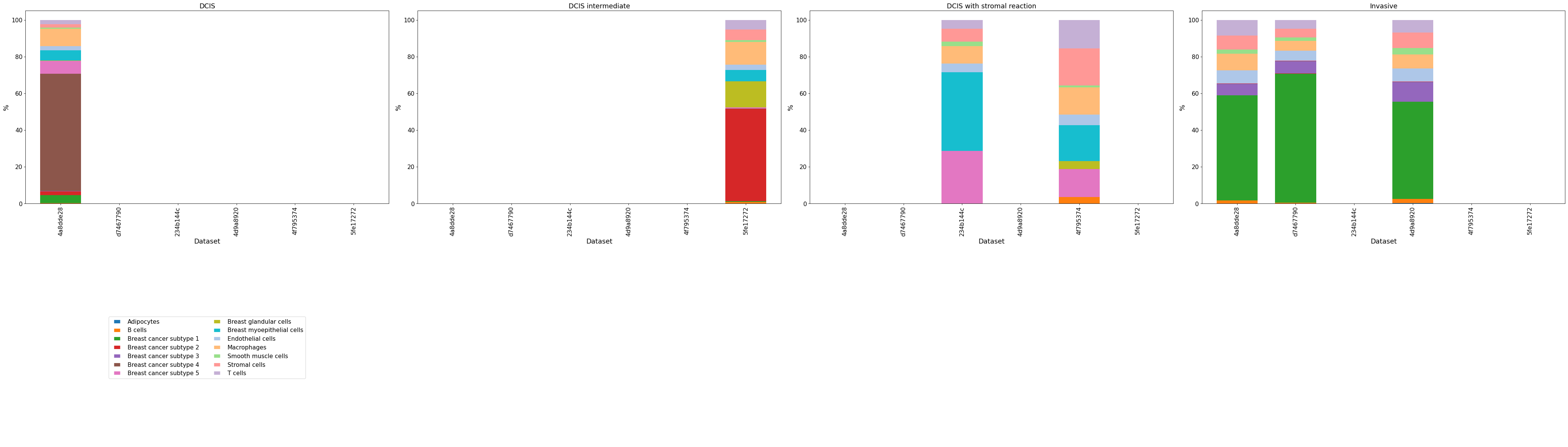
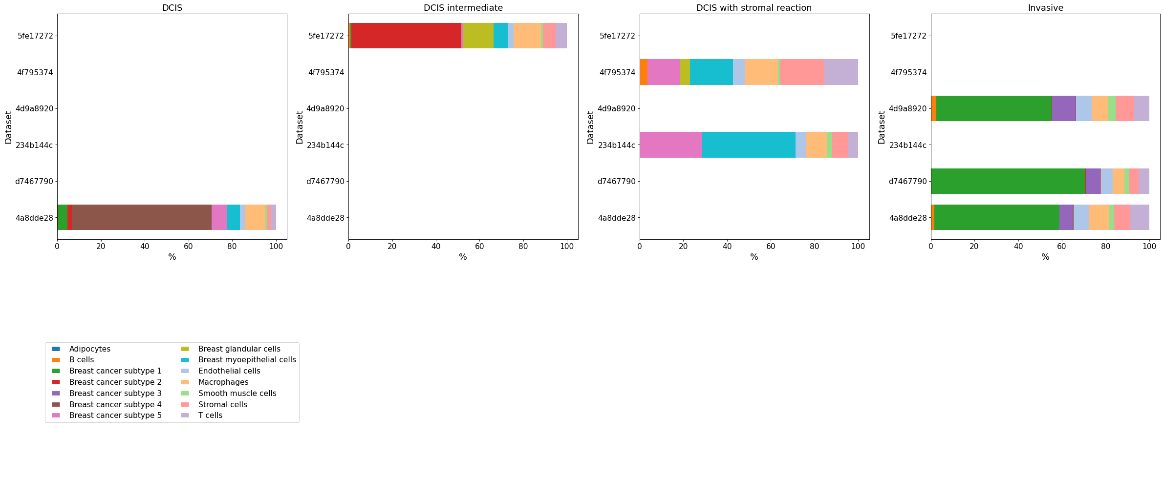
If a geom_key together with an InSituExperiment object are given, the datasets are compared against each other per geometry. If a dataset does not contain one of the geometries, the bar stays empty.
cellular_composition(
    data=exp, cell_type_col="cell_type_dc_sub_final",
    geom_key="Katja", modality="annotations", max_cols=4,
    legend_max_per_col=10,
    #savepath="figures/cell_composition_regions_Demo_publ.pdf"
)
Whether to use a vertical or horizontal bar plot can be specified using plot_type. The dimensions of the bar plots can be changed using the aspect_factor argument. The legend can be adapted using legend_max_per_col.
cellular_composition(
    data=exp, cell_type_col="cell_type_dc_sub_final",
    geom_key="Katja", modality="annotations", max_cols=4,
    plot_type="bar", aspect_factor=0.5,
    legend_max_per_col=10,
    #savepath="figures/cell_composition_regions_Demo_publ.pdf"
)