Spatial plotting functionalities

This notebook shows the insitupy plotting functionalities. It assumes that the previous steps of the demo notebooks such as preprocessing, import of annotations and regions and cell type annotation have been run.

## The following code ensures that all functions and init files are reloaded before executions.
%load_ext autoreload
%autoreload 2

from pathlib import Path
from insitupy import InSituData, CACHE

Load data

insitupy_project = Path(CACHE / "out/demo_insitupy_project")
xd = InSituData.read(insitupy_project)
xd.load_all()

xd

InSituData
Method:		Xenium
Slide ID:	0001879
Sample ID:	Replicate 1
Path:		C:\Users\ge37voy\.cache\InSituPy\out\demo_insitupy_project
Metadata file:	.ispy
    ➤ images
       nuclei:	(25778, 35416)
       CD20:	(25778, 35416)
       HER2:	(25778, 35416)
       HE:	(25778, 35416, 3)
    ➤ cells
       MultiCellData with main layer 'main'
           matrix
               AnnData object with n_obs × n_vars = 156447 × 297
               obs: 'transcript_counts', 'control_probe_counts', 'control_codeword_counts', 'total_counts', 'cell_area', 'nucleus_area', 'n_genes_by_counts', 'n_genes', 'leiden', 'cell_type_dc', 'cell_type_dc_sub', 'cell_type_tacco', 'cell_type_publ'
               var: 'gene_ids', 'feature_types', 'genome', 'n_cells_by_counts', 'mean_counts', 'pct_dropout_by_counts', 'total_counts', 'n_cells'
               uns: 'cell_type_dc_colors', 'cell_type_dc_sub', 'cell_type_dc_sub_colors', 'cell_type_publ_colors', 'cell_type_tacco_colors', 'counts_location', 'leiden', 'leiden_colors', 'log1p', 'neighbors', 'pca', 'umap'
               obsm: 'OT', 'X_pca', 'X_umap', 'annotations', 'ora_estimate', 'ora_pvals', 'regions', 'spatial'
               varm: 'OT', 'PCs'
               layers: 'counts', 'norm_counts'
               obsp: 'connectivities', 'distances'
           boundaries
               BoundariesData object with 2 entries:
                   cells
                   nuclei
    ➤ transcripts
       DataFrame with shape <dask_expr.expr.Scalar: expr=ReadParquetFSSpec(184a915).size() // 8, dtype=int64> x 8
    ➤ annotations
       TestKey:	9 annotations, 2 classes ('TestClass','points') ✔
       demo:	4 annotations, 1 class ('None') ✔
       demo2:	5 annotations, 1 class ('None') ✔
       demo3:	7 annotations, 1 class ('None') ✔
       Demo:	28 annotations, 2 classes ('Tumor cells','Stroma') ✔
    ➤ regions
       demo_regions:	3 regions, 3 classes ('Region1','Region2','Region3') ✔
       TMA:	6 regions, 6 classes ('B-2','A-3','B-1','B-3','A-1','A-2') ✔
       Demo:	3 regions, 3 classes ('Region 1','Region 3','Region 2') ✔

Sample-level or experimental level plotting of expression data

from insitupy.plotting import plot_spatial

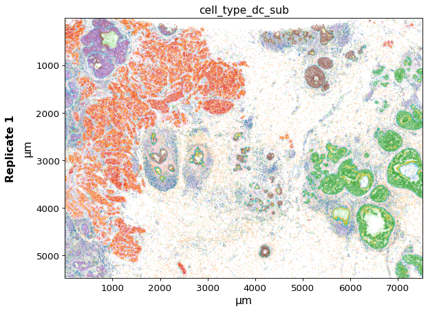
Using the keys argument, one or multiple keys can be selected to be displayed.

plot_spatial(xd, keys="cell_type_dc_sub")

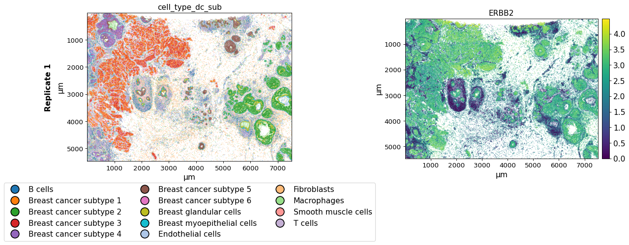
plot_spatial(xd, keys=["cell_type_dc_sub", "ERBB2"])

The savepath argument can be used to save the plot in a certain path. The filename extension determines the format of the output image. When saving as .pdf long saving times can occur due to the large number of data points.

plot_spatial(xd, keys=["cell_type_dc_sub", "ERBB2"],
             savepath="figures/spatial-demo.png")

Saving figure to file figures/spatial-demo.png
Saved.

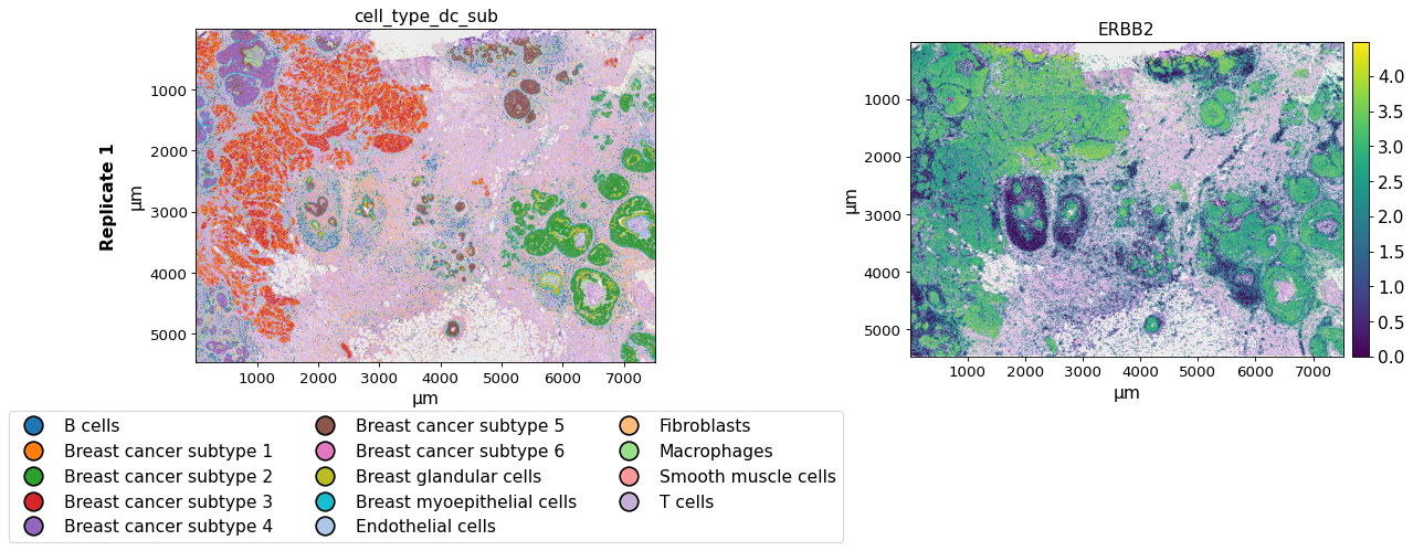
The image_key argument can be used to select a image to be displayed in the background.

plot_spatial(xd, keys=["cell_type_dc_sub", "ERBB2"],
             image_key="HE",
             )

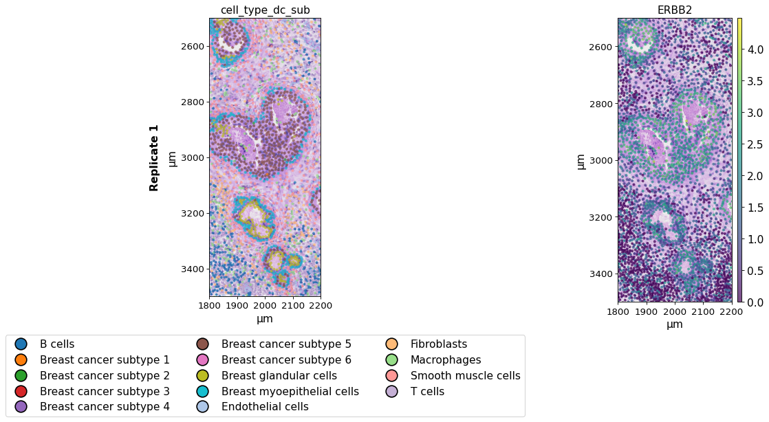
The xlim/ylim parameters can be used to zoom into the images and plot only selected regions and the spot_size argument to adapt the size of the spots. Further, the opacity of the spots can be adapted using alpha.

plot_spatial(xd, keys=["cell_type_dc_sub", "ERBB2"],
             spot_size=8, alpha=0.7,
             xlim=(1800, 2200), ylim=(2500, 3500),
             image_key="HE",
             )

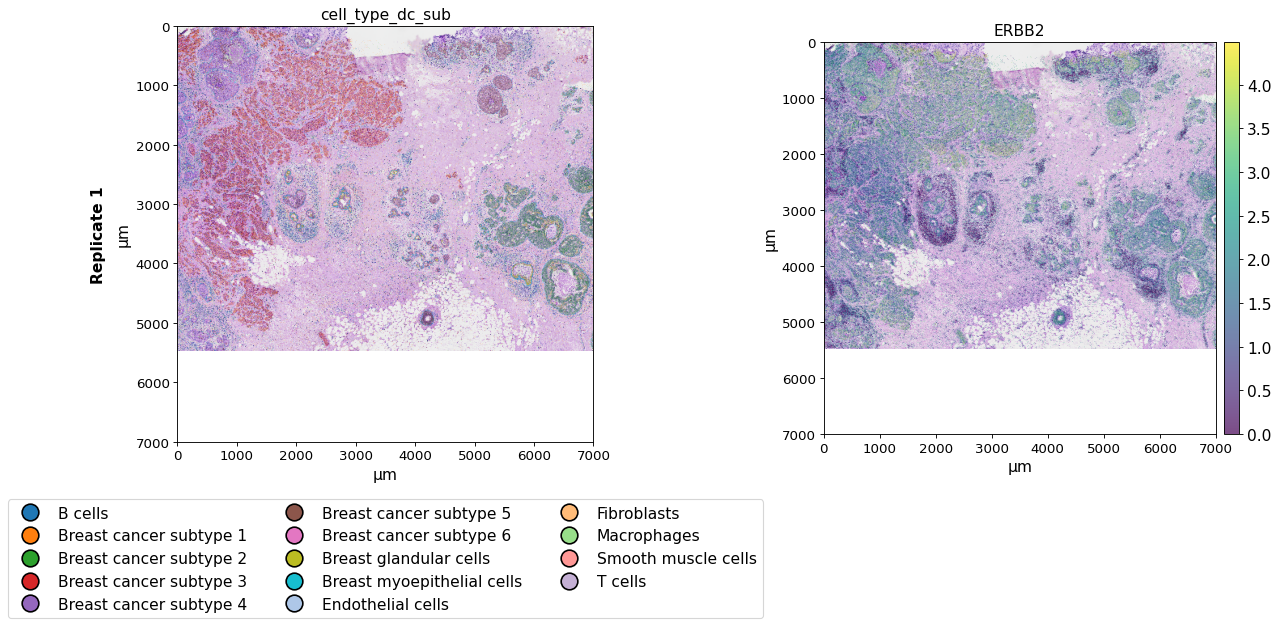
plot_spatial(xd, keys=["cell_type_dc_sub", "ERBB2"],
             spot_size=8, alpha=0.7,
             xlim=(0, 7000), ylim=(0, 7000),
             image_key="HE",
             )

When working with an InSituExperiment object for multi-sample analysis, one can directly plot all datasets within the InSituExperiment object. For details on generating InSituExperiment objects and working with them see this notebook.

from insitupy import InSituExperiment

First, we generate an InSituExperiment object.

exp = InSituExperiment.from_regions(
    data=xd, region_key="TMA"
)

A-1
A-2
A-3
B-1
B-2
B-3

And then we can use the plot_spatial function directly on the InSituExperiment object. The name_column argument can be used to determine the column in the .metadata dataframe to be used for naming the plot.

exp.metadata

	uid	slide_id	sample_id	region_key	region_name
0	39abd0f9	0001879	Replicate 1	TMA	A-1
1	a4b97164	0001879	Replicate 1	TMA	A-2
2	bb7d859e	0001879	Replicate 1	TMA	A-3
3	b2580297	0001879	Replicate 1	TMA	B-1
4	ba9b5f9e	0001879	Replicate 1	TMA	B-2
5	80290f88	0001879	Replicate 1	TMA	B-3

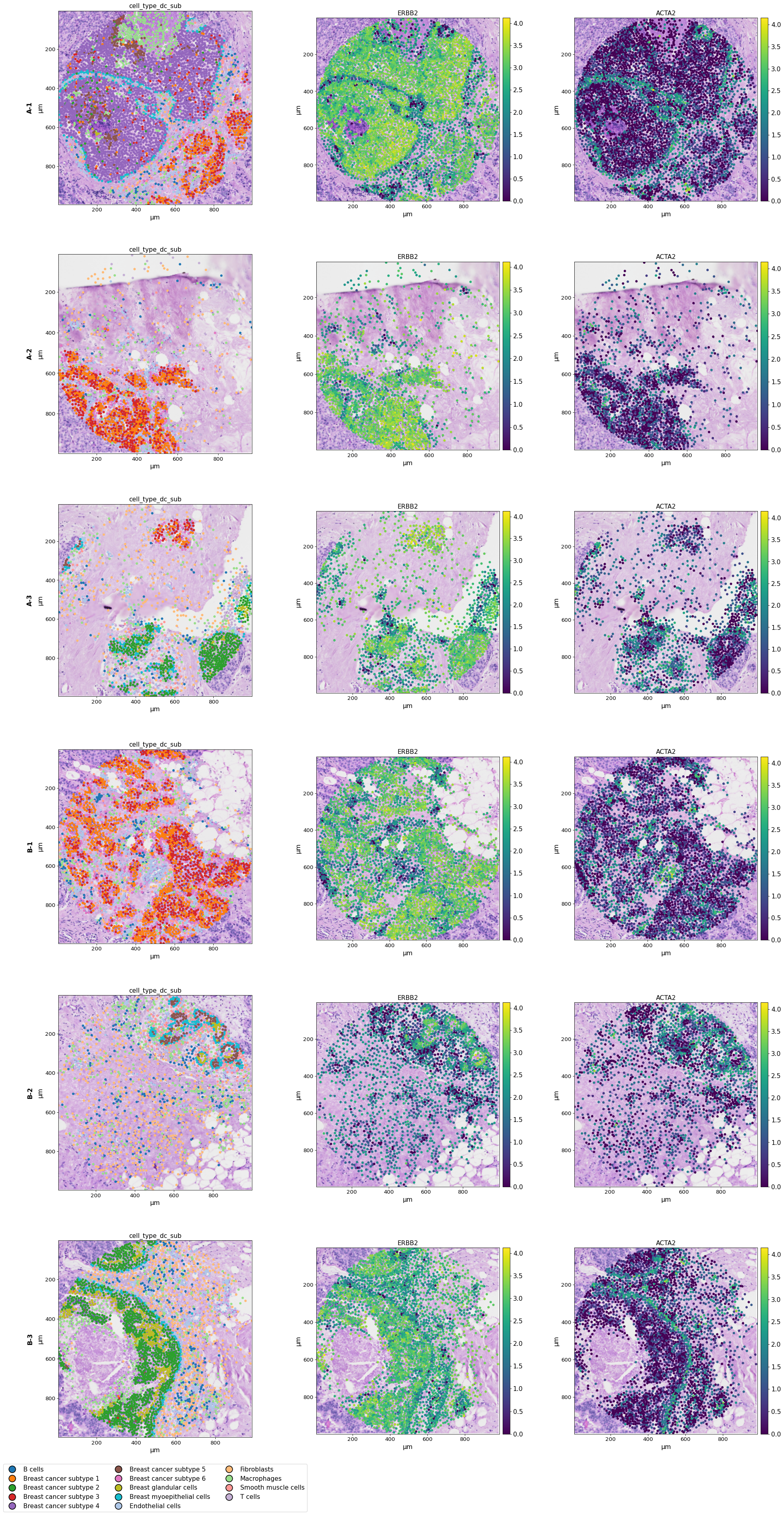
When using both multiple datasets and multiple keys the plots are represented in a grid layout.

plot_spatial(exp, keys=["cell_type_dc_sub", "ERBB2", "ACTA2"], image_key="HE",
             name_column="region_name")

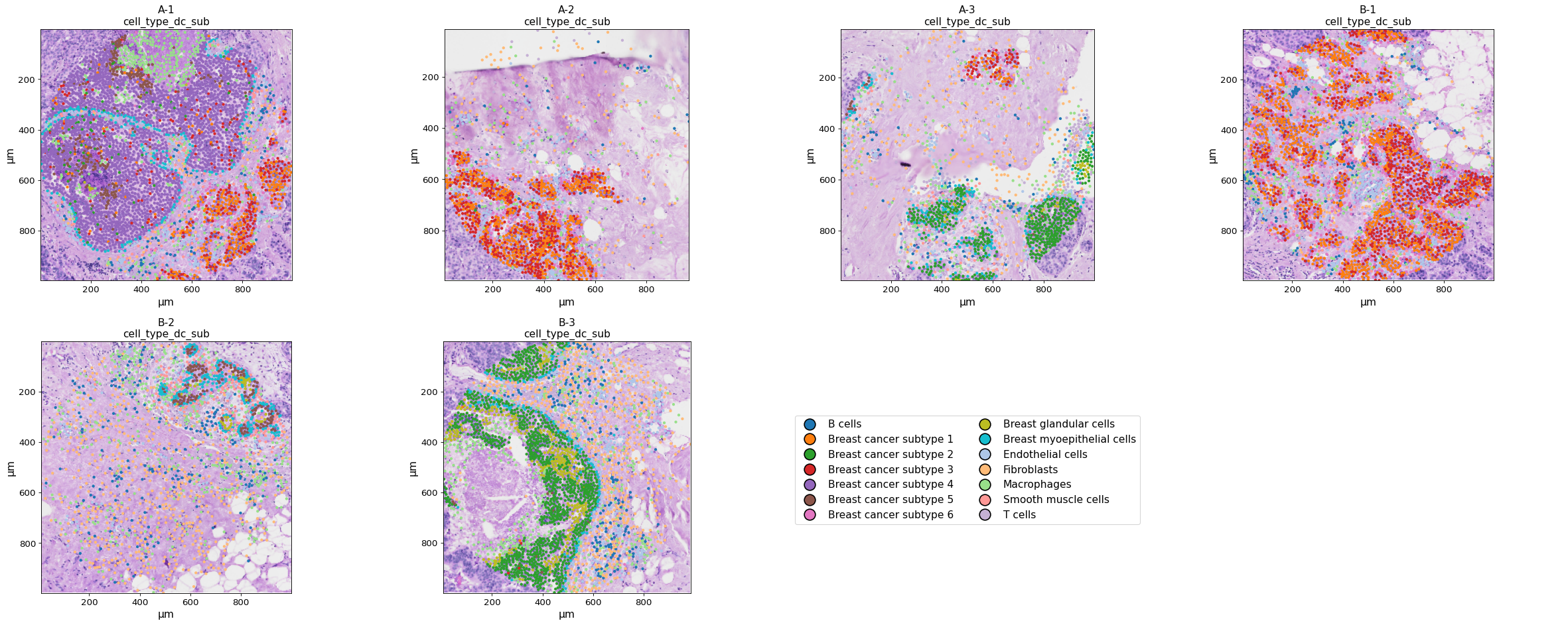
When using only multiple datasets but only one key, they are listed next to each other.

plot_spatial(exp, keys=["cell_type_dc_sub"], image_key="HE",
             name_column="region_name")