Investigate gene expression and cell density along an axis#
## The following code ensures that all functions and init files are reloaded before executions.
%load_ext autoreload
%autoreload 2
from pathlib import Path
from insitupy import InSituData, CACHE
import warnings
warnings.simplefilter(action='ignore', category=FutureWarning)
Load Xenium data into InSituData object#
Now the Xenium data can be parsed by providing the data path to the InSituPy project folder.
insitupy_project = Path(CACHE / "out/demo_insitupy_project")
xd = InSituData.read(insitupy_project)
xd.load_all()
xd
InSituData
Method:		Xenium
Slide ID:	0001879
Sample ID:	Replicate 1
Path:		C:\Users\ge37voy\.cache\InSituPy\out\demo_insitupy_project

    ➤ images
       CD20:	(25778, 35416)
       HE:	(25778, 35416, 3)
       HER2:	(25778, 35416)
       nuclei:	(25778, 35416)
    ➤ cells
       MultiCellData with main layer 'main'
           matrix
               AnnData object with n_obs × n_vars = 156447 × 297
               obs: 'transcript_counts', 'control_probe_counts', 'control_codeword_counts', 'total_counts', 'cell_area', 'nucleus_area', 'n_genes_by_counts', 'n_genes', 'leiden', 'cell_type_dc_sub_final', 'cell_type_publ'
               var: 'gene_ids', 'feature_types', 'genome', 'n_cells_by_counts', 'mean_counts', 'pct_dropout_by_counts', 'total_counts', 'n_cells'
               uns: 'cell_type_dc_sub_final_colors', 'cell_type_publ_colors', 'leiden', 'leiden_colors', 'log1p', 'neighbors', 'pca', 'umap'
               obsm: 'X_pca', 'X_umap', 'annotations', 'regions', 'spatial'
               varm: 'PCs'
               layers: 'counts', 'norm_counts'
               obsp: 'connectivities', 'distances'
           boundaries
               BoundariesData object with 2 entries:
                   cells
                   nuclei
    ➤ transcripts
       DataFrame with shape <dask_expr.expr.Scalar: expr=ReadParquetFSSpec(7603627).size() // 8, dtype=int64> x 8
    ➤ annotations
       TestKey:	3 annotations, 1 class ('TestClass') ✔
       test:	6 annotations, 1 class ('testclass') ✔
       demo:	28 annotations, 2 classes ('Stroma', 'Tumor cells') ✔
       demo2:	5 annotations, 3 classes ('Negative', 'Other', 'Positive') ✔
       demo3:	7 annotations, 5 classes ('Immune cells', 'Necrosis', 'Stroma', 'Tumor', 'unclassified') ✔
       Demo:	28 annotations, 2 classes ('Stroma', 'Tumor cells') ✔
       Janesick:	18 annotations, 3 classes ('DCIS #1', 'DCIS #2', 'Invasive')
       Katja:	18 annotations, 4 classes ('DCIS', 'DCIS intermediate', 'DCIS with stromal reaction', 'Invasive') ✔
    ➤ regions
       demo_regions:	3 regions, 3 classes ('Region1', 'Region2', 'Region3') ✔
       TMA:	6 regions, 6 classes ('A-1', 'A-2', 'A-3', 'B-1', 'B-2', 'B-3') ✔
       Demo:	3 regions, 3 classes ('Region 1', 'Region 2', 'Region 3') ✔
       Katja:	4 regions, 4 classes ('Region 1', 'Region 2', 'Region 3', 'Region 4')
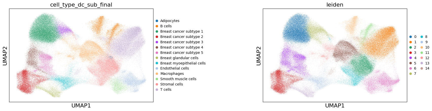
import scanpy as sc
sc.pl.umap(adata=xd.cells.matrix, color=["cell_type_dc_sub_final", "leiden"], wspace=0.6)
Import annotations#
xd.import_annotations(
    files=["../../demo_data/demo_annotations/annotations-Tumor.geojson",
           "../../demo_data/demo_annotations/demo_annotations.geojson",
           "../../demo_data/demo_annotations/demo_points.geojson"],
    keys=["Tumor", "Demo", "Demo"],
    scale_factor=0.2125
)

xd.import_regions(
    files="../../demo_data/demo_regions/regions-Tumor.geojson",
    keys="Tumor",
    scale_factor=0.2125
)
Select small region for demonstration purposes#
xdcrop = xd.crop(region_tuple=("Tumor", "Selected Tumor"))

# access transcriptomic data in anndata format from InSituData object
adata = xdcrop.cells.matrix
Calculate density using kernel density estimation or Mellon#
The kernel density can be used to identify regions with an increased density of a certain cell type (e.g. immune cells).
from insitupy.utils._calc import calc_density
Option 1: Kernel density estimation#
# Example usage using gaussian kernel density estimation
calc_density(
    adata,
    groupby='cell_type_dc_sub_final',
    mode="gauss",
    inplace=True)
Option 2: Mellon package#
# Example usage using mellon density estimation
calc_density(
    adata,
    groupby='cell_type_dc_sub_final',
    mode="mellon",
    inplace=True)
[2025-11-05 21:00:14,344] [INFO    ] Using sparse Gaussian Process since n_landmarks (5,000) < n_samples (5,237) and rank = 1.0.
[2025-11-05 21:00:14,360] [INFO    ] Computing nearest neighbor distances.
[2025-11-05 21:00:54,598] [INFO    ] Using embedding dimensionality d=2. Use d_method="fractal" to enable effective density normalization.
[2025-11-05 21:00:55,244] [INFO    ] Using covariance function Matern52(ls=322.3459167480469).
[2025-11-05 21:00:55,246] [INFO    ] Computing 5,000 landmarks with k-means clustering (random_state=42).
[2025-11-05 21:01:05,271] [INFO    ] Using rank 5,000 covariance representation.
[2025-11-05 21:01:07,840] [INFO    ] Running inference using L-BFGS-B.
[2025-11-05 21:01:11,555] [INFO    ] Using non-sparse Gaussian Process since n_landmarks (2,651) >= n_samples (2,651) and rank = 1.0.
[2025-11-05 21:01:11,557] [INFO    ] Computing nearest neighbor distances.
[2025-11-05 21:01:12,109] [INFO    ] Using embedding dimensionality d=2. Use d_method="fractal" to enable effective density normalization.
[2025-11-05 21:01:12,413] [INFO    ] Using covariance function Matern52(ls=280.4144287109375).
[2025-11-05 21:01:12,416] [INFO    ] Computing Lp.
[2025-11-05 21:01:13,823] [INFO    ] Using rank 2,651 covariance representation.
[2025-11-05 21:01:14,488] [INFO    ] Running inference using L-BFGS-B.
[2025-11-05 21:01:16,434] [INFO    ] Using non-sparse Gaussian Process since n_landmarks (2,954) >= n_samples (2,954) and rank = 1.0.
[2025-11-05 21:01:16,434] [INFO    ] Computing nearest neighbor distances.
[2025-11-05 21:01:16,964] [INFO    ] Using embedding dimensionality d=2. Use d_method="fractal" to enable effective density normalization.
[2025-11-05 21:01:17,299] [INFO    ] Using covariance function Matern52(ls=333.7417907714844).
[2025-11-05 21:01:17,299] [INFO    ] Computing Lp.
[2025-11-05 21:01:18,798] [INFO    ] Using rank 2,954 covariance representation.
[2025-11-05 21:01:19,494] [INFO    ] Running inference using L-BFGS-B.
[2025-11-05 21:01:21,658] [INFO    ] Using sparse Gaussian Process since n_landmarks (5,000) < n_samples (5,763) and rank = 1.0.
[2025-11-05 21:01:21,661] [INFO    ] Computing nearest neighbor distances.
[2025-11-05 21:01:22,242] [INFO    ] Using embedding dimensionality d=2. Use d_method="fractal" to enable effective density normalization.
[2025-11-05 21:01:22,552] [INFO    ] Using covariance function Matern52(ls=226.2815704345703).
[2025-11-05 21:01:22,552] [INFO    ] Computing 5,000 landmarks with k-means clustering (random_state=42).
[2025-11-05 21:01:29,825] [INFO    ] Using rank 5,000 covariance representation.
[2025-11-05 21:01:32,459] [INFO    ] Running inference using L-BFGS-B.
[2025-11-05 21:01:35,864] [INFO    ] Using non-sparse Gaussian Process since n_landmarks (108) >= n_samples (108) and rank = 1.0.
[2025-11-05 21:01:35,866] [INFO    ] Computing nearest neighbor distances.
[2025-11-05 21:01:36,371] [INFO    ] Using embedding dimensionality d=2. Use d_method="fractal" to enable effective density normalization.
[2025-11-05 21:01:36,699] [INFO    ] Using covariance function Matern52(ls=209.92318725585938).
[2025-11-05 21:01:36,701] [INFO    ] Computing Lp.
[2025-11-05 21:01:37,918] [INFO    ] Using rank 108 covariance representation.
[2025-11-05 21:01:38,069] [INFO    ] Running inference using L-BFGS-B.
[2025-11-05 21:01:39,105] [INFO    ] Using non-sparse Gaussian Process since n_landmarks (47) >= n_samples (47) and rank = 1.0.
[2025-11-05 21:01:39,105] [INFO    ] Computing nearest neighbor distances.
[2025-11-05 21:01:39,597] [INFO    ] Using embedding dimensionality d=2. Use d_method="fractal" to enable effective density normalization.
[2025-11-05 21:01:39,979] [INFO    ] Using covariance function Matern52(ls=351.9698181152344).
[2025-11-05 21:01:39,982] [INFO    ] Computing Lp.
[2025-11-05 21:01:41,091] [INFO    ] Using rank 47 covariance representation.
[2025-11-05 21:01:41,258] [INFO    ] Running inference using L-BFGS-B.
[2025-11-05 21:01:42,424] [INFO    ] Using non-sparse Gaussian Process since n_landmarks (1,392) >= n_samples (1,392) and rank = 1.0.
[2025-11-05 21:01:42,424] [INFO    ] Computing nearest neighbor distances.
[2025-11-05 21:01:42,940] [INFO    ] Using embedding dimensionality d=2. Use d_method="fractal" to enable effective density normalization.
[2025-11-05 21:01:43,225] [INFO    ] Using covariance function Matern52(ls=183.39097595214844).
[2025-11-05 21:01:43,238] [INFO    ] Computing Lp.
[2025-11-05 21:01:44,441] [INFO    ] Using rank 1,392 covariance representation.
[2025-11-05 21:01:44,688] [INFO    ] Running inference using L-BFGS-B.
[2025-11-05 21:01:46,304] [INFO    ] Using non-sparse Gaussian Process since n_landmarks (1,680) >= n_samples (1,680) and rank = 1.0.
[2025-11-05 21:01:46,306] [INFO    ] Computing nearest neighbor distances.
[2025-11-05 21:01:46,801] [INFO    ] Using embedding dimensionality d=2. Use d_method="fractal" to enable effective density normalization.
[2025-11-05 21:01:47,092] [INFO    ] Using covariance function Matern52(ls=203.98988342285156).
[2025-11-05 21:01:47,096] [INFO    ] Computing Lp.
[2025-11-05 21:01:48,563] [INFO    ] Using rank 1,680 covariance representation.
[2025-11-05 21:01:48,873] [INFO    ] Running inference using L-BFGS-B.
[2025-11-05 21:01:50,642] [INFO    ] Using non-sparse Gaussian Process since n_landmarks (871) >= n_samples (871) and rank = 1.0.
[2025-11-05 21:01:50,644] [INFO    ] Computing nearest neighbor distances.
[2025-11-05 21:01:51,140] [INFO    ] Using embedding dimensionality d=2. Use d_method="fractal" to enable effective density normalization.
[2025-11-05 21:01:51,432] [INFO    ] Using covariance function Matern52(ls=305.643310546875).
[2025-11-05 21:01:51,432] [INFO    ] Computing Lp.
[2025-11-05 21:01:52,734] [INFO    ] Using rank 871 covariance representation.
[2025-11-05 21:01:52,937] [INFO    ] Running inference using L-BFGS-B.
[2025-11-05 21:01:54,456] [INFO    ] Using non-sparse Gaussian Process since n_landmarks (662) >= n_samples (662) and rank = 1.0.
[2025-11-05 21:01:54,459] [INFO    ] Computing nearest neighbor distances.
[2025-11-05 21:01:54,974] [INFO    ] Using embedding dimensionality d=2. Use d_method="fractal" to enable effective density normalization.
[2025-11-05 21:01:55,354] [INFO    ] Using covariance function Matern52(ls=178.8740997314453).
[2025-11-05 21:01:55,357] [INFO    ] Computing Lp.
[2025-11-05 21:01:56,698] [INFO    ] Using rank 662 covariance representation.
[2025-11-05 21:01:56,889] [INFO    ] Running inference using L-BFGS-B.
[2025-11-05 21:01:58,921] [INFO    ] Using non-sparse Gaussian Process since n_landmarks (317) >= n_samples (317) and rank = 1.0.
[2025-11-05 21:01:58,924] [INFO    ] Computing nearest neighbor distances.
[2025-11-05 21:01:59,452] [INFO    ] Using embedding dimensionality d=2. Use d_method="fractal" to enable effective density normalization.
[2025-11-05 21:01:59,861] [INFO    ] Using covariance function Matern52(ls=406.76336669921875).
[2025-11-05 21:01:59,863] [INFO    ] Computing Lp.
[2025-11-05 21:02:01,208] [INFO    ] Using rank 317 covariance representation.
[2025-11-05 21:02:01,368] [INFO    ] Running inference using L-BFGS-B.
[2025-11-05 21:02:02,693] [INFO    ] Using non-sparse Gaussian Process since n_landmarks (12) >= n_samples (12) and rank = 1.0.
[2025-11-05 21:02:02,696] [INFO    ] Computing nearest neighbor distances.
[2025-11-05 21:02:03,093] [INFO    ] Using embedding dimensionality d=2. Use d_method="fractal" to enable effective density normalization.
[2025-11-05 21:02:03,316] [INFO    ] Using covariance function Matern52(ls=1956.1572265625).
[2025-11-05 21:02:03,316] [INFO    ] Computing Lp.
[2025-11-05 21:02:04,447] [INFO    ] Using rank 12 covariance representation.
[2025-11-05 21:02:04,597] [INFO    ] Running inference using L-BFGS-B.
[2025-11-05 21:02:05,668] [INFO    ] Using non-sparse Gaussian Process since n_landmarks (6) >= n_samples (6) and rank = 1.0.
[2025-11-05 21:02:05,671] [INFO    ] Computing nearest neighbor distances.
[2025-11-05 21:02:06,134] [INFO    ] Using embedding dimensionality d=2. Use d_method="fractal" to enable effective density normalization.
[2025-11-05 21:02:06,397] [INFO    ] Using covariance function Matern52(ls=4851.75048828125).
[2025-11-05 21:02:06,400] [INFO    ] Computing Lp.
[2025-11-05 21:02:07,551] [INFO    ] Using rank 6 covariance representation.
[2025-11-05 21:02:07,709] [INFO    ] Running inference using L-BFGS-B.
[2025-11-05 21:02:08,741] [INFO    ] Using non-sparse Gaussian Process since n_landmarks (11) >= n_samples (11) and rank = 1.0.
[2025-11-05 21:02:08,743] [INFO    ] Computing nearest neighbor distances.
[2025-11-05 21:02:09,062] [INFO    ] Using embedding dimensionality d=2. Use d_method="fractal" to enable effective density normalization.
[2025-11-05 21:02:09,227] [INFO    ] Using covariance function Matern52(ls=4877.8056640625).
[2025-11-05 21:02:09,229] [INFO    ] Computing Lp.
[2025-11-05 21:02:09,902] [INFO    ] Using rank 11 covariance representation.
[2025-11-05 21:02:09,995] [INFO    ] Running inference using L-BFGS-B.
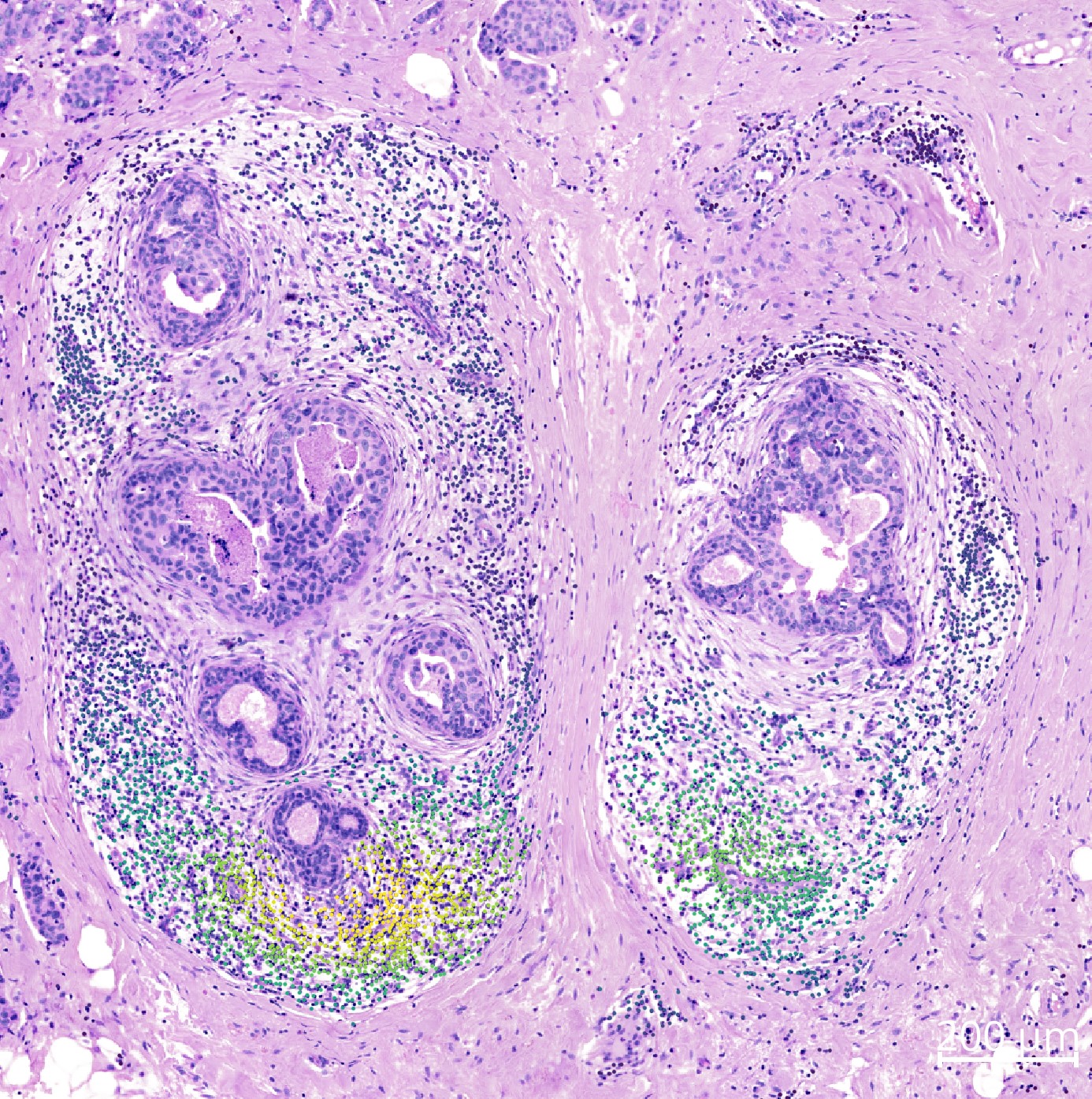
The results are saved in .cells.matrix.obsm["density-{method}'] and can be viewed using .show().
xdcrop.show()
Below is the result if you select following:
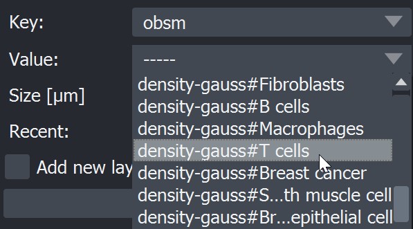
Result:
Visualize effects along an axis#
Alternatively to visualizing the cellular gene expression or density in 2D as shown above, it is also possible to visualize it along an axis. In the example scenario below we calculate the distance of each cell to the tumor center and visualize the cellular density and gene expression along this axis.
Calculate distance of cells to annotations#
To generate an axis we use here a selected set of annotations and calculate the distance of all cells to these annotations. For demonstration purposes we selected a region of the breast cancer dataset and annotated tumor cells within this region:
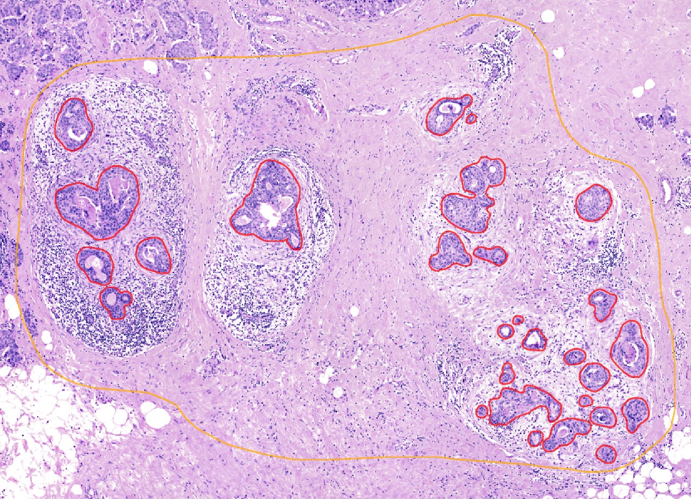 These annotations and the region can be imported from files in the repository but of course it would be also possible to do own annotations and select an own region and save the results using
 .store_geometries().
from insitupy.tools import calc_distance_of_cells_from
calc_distance_of_cells_from(
    data=xdcrop,
    annotation_key="Demo",
    annotation_class="Tumor center",
    # region_key="Tumor",
    # region_name="Selected Tumor"
)
Using CellData from MultiCellData layer 'main'.
Calculate the distance of cells from the annotation "Tumor center"
Saved distances to `.cells[main].matrix.obsm["distance_from"]["Tumor center"]`
The distances can be accessed in .cells.matrix.obsm["distance_from"]
xdcrop.cells.matrix.obsm["distance_from"]
| Tumor center | |
|---|---|
| 4353 | 231.644821 |
| 4356 | 226.342973 |
| 4358 | 213.661463 |
| 4359 | 216.604613 |
| 4390 | 226.413766 |
| ... | ... |
| 118567 | 135.302369 |
| 118569 | 156.354595 |
| 118570 | 162.485566 |
| 118575 | 147.131136 |
| 118576 | 164.307876 |
21711 rows × 1 columns
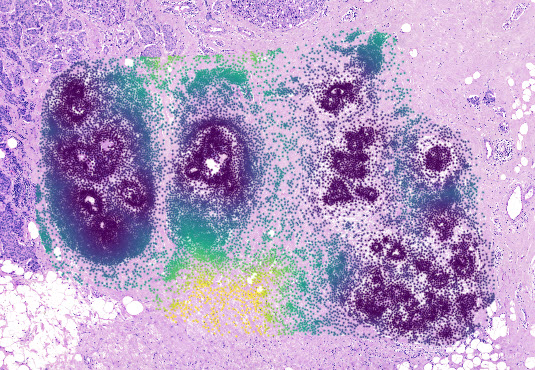
Visualize the results using napari#
Using .show() we can visualize the results and see the distance values per cell:
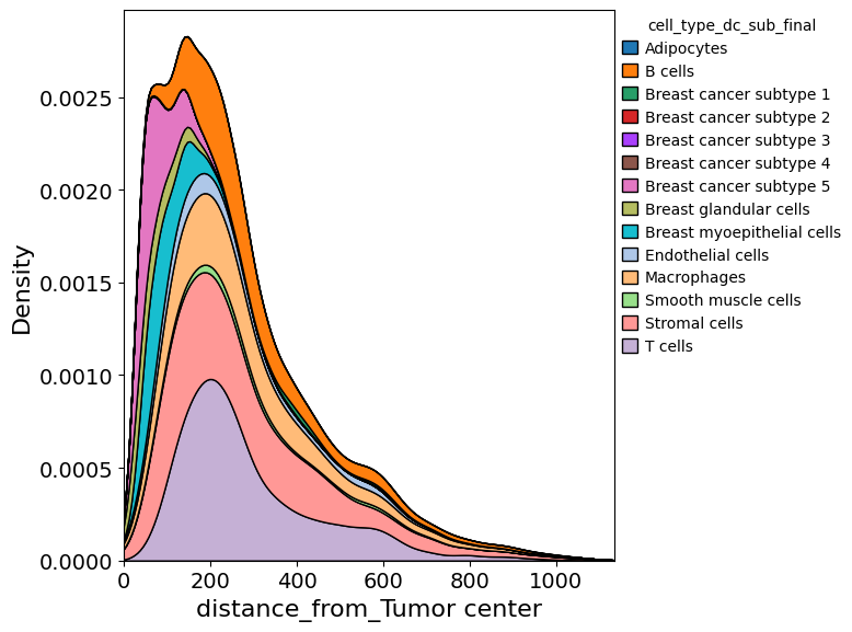
Plot cell abundance along axis#
In addition to exploring the density of a certain cell type in two dimension, one can also explore it along a certain axis.
from insitupy.plotting import cell_abundance_along_axis
"cell_type_dc_colors" in xdcrop.cells.matrix.uns
False
cell_abundance_along_axis(
    adata=xdcrop.cells.matrix,
    axis=("distance_from", "Tumor center"),
    groupby="cell_type_dc_sub_final",
    kde=True
)
Retrieve axis from `.obsm`.
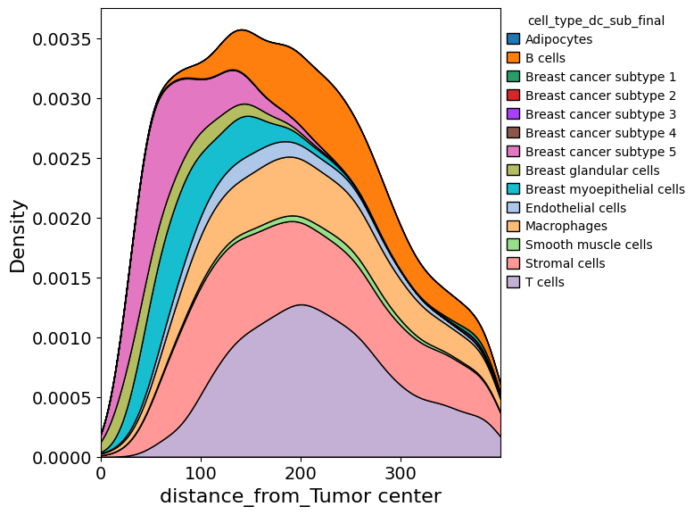
cell_abundance_along_axis(
    adata=xdcrop.cells.matrix,
    axis=("distance_from", "Tumor center"),
    groupby="cell_type_dc_sub_final",
    xlim=(0,400),
    kde=True,
    savepath="figures/cell_abundance_along_axis.pdf"
)
Retrieve axis from `.obsm`.
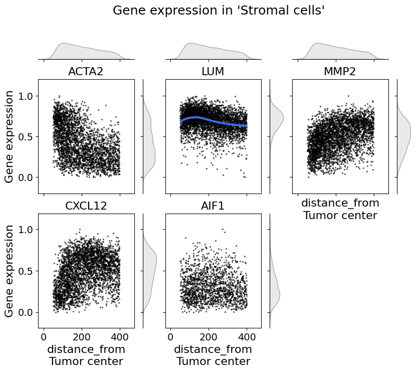
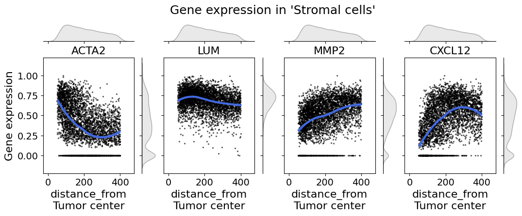
Explore cellular density and gene expression along axis#
In single-cell spatial transcriptomic data it is important to explore the gene expression on a cell type level. The cell_expression_along_axis function let’s you do so.
from insitupy.plotting import cell_expression_along_axis

# Example usage:
cell_expression_along_axis(
    adata=xdcrop.cells.matrix,
    axis=("distance_from", "Tumor center"),
    cell_type_column="cell_type_dc_sub_final",
    cell_type="Stromal cells",
    genes=["ACTA2", "LUM", "MMP2", "CXCL12"],
    xlim=(50, 400),
    kde=False,
    fit_reg=True,
    min_expression=0,
    savepath="figures/gene_expr_along_axis_Stromal cells.pdf"
    )
Number of columns to plot can be changed with the max_cols argument:
from insitupy.plotting import cell_expression_along_axis

# Example usage:
cell_expression_along_axis(
    adata=xdcrop.cells.matrix,
    axis=("distance_from", "Tumor center"),
    cell_type_column="cell_type_dc_sub_final",
    cell_type="Stromal cells",
    genes=["ACTA2", "LUM", "MMP2", "CXCL12", "AIF1"],
    max_cols=3,
    xlim=(50, 400),
    kde=False,
    fit_reg=True,
    min_expression=0.1,
    #savepath="figures/gene_expr_along_axis_fibroblasts.pdf"
    )